Three Gates and Seven Buckets: What Frontier Labs Actually Test
Table of Contents
- The thing that gets you in stops working once you are in
- Gate 1: getting seen
- The shape of the loop
- Bucket 1: Progressive system building
- Bucket 2: ML coding
- Bucket 3: AI fundamentals
- Bucket 4: Training schemes and mechanisms
- Bucket 5: ML systems design
- Bucket 6: Research taste, deep dives, and values
- Bucket 7: Math
- Gate 3: timing, work trials, and negotiation
- The part nobody prepares for
- Sequencing your preparation
- What I would still get wrong
- References
The thing that gets you in stops working once you are in
Three people who joined frontier labs in 2026 wrote up their job searches within about a month of each other. They worked in different subfields, interviewed at different companies, and wrote in different registers. They say the same thing.
Alisa Liu, who finished a six-year NLP PhD at the University of Washington and is now a Research Scientist at OpenAI, puts it most precisely:
“Overall, technical skills and knowledge are evaluated much more than research experience, though the latter probably gets you the interview in the first place.” [30]
Silvia Sapora, who went from an ML PhD to Research Scientist at Google DeepMind, puts it more bluntly:
“if you’re already getting interviews: more papers will not help you at this point. You need to pass the interviews, and often the people interviewing you won’t even look at your CV. So, stop focusing on your research and your papers, and start focusing on interview prep!” [42]
And Yong Zheng-Xin, a Brown PhD who pivoted from multilingual NLP into AI safety mid-search, found that only one or two papers mattered at all — “Sometimes, none at all, and I was just being evaluated on how well I solve the team’s problems on the spot” [55].
That is the structure of this whole thing. It is not one test. It is three, in sequence, and the currency that buys you passage through one gate is worthless at the next.
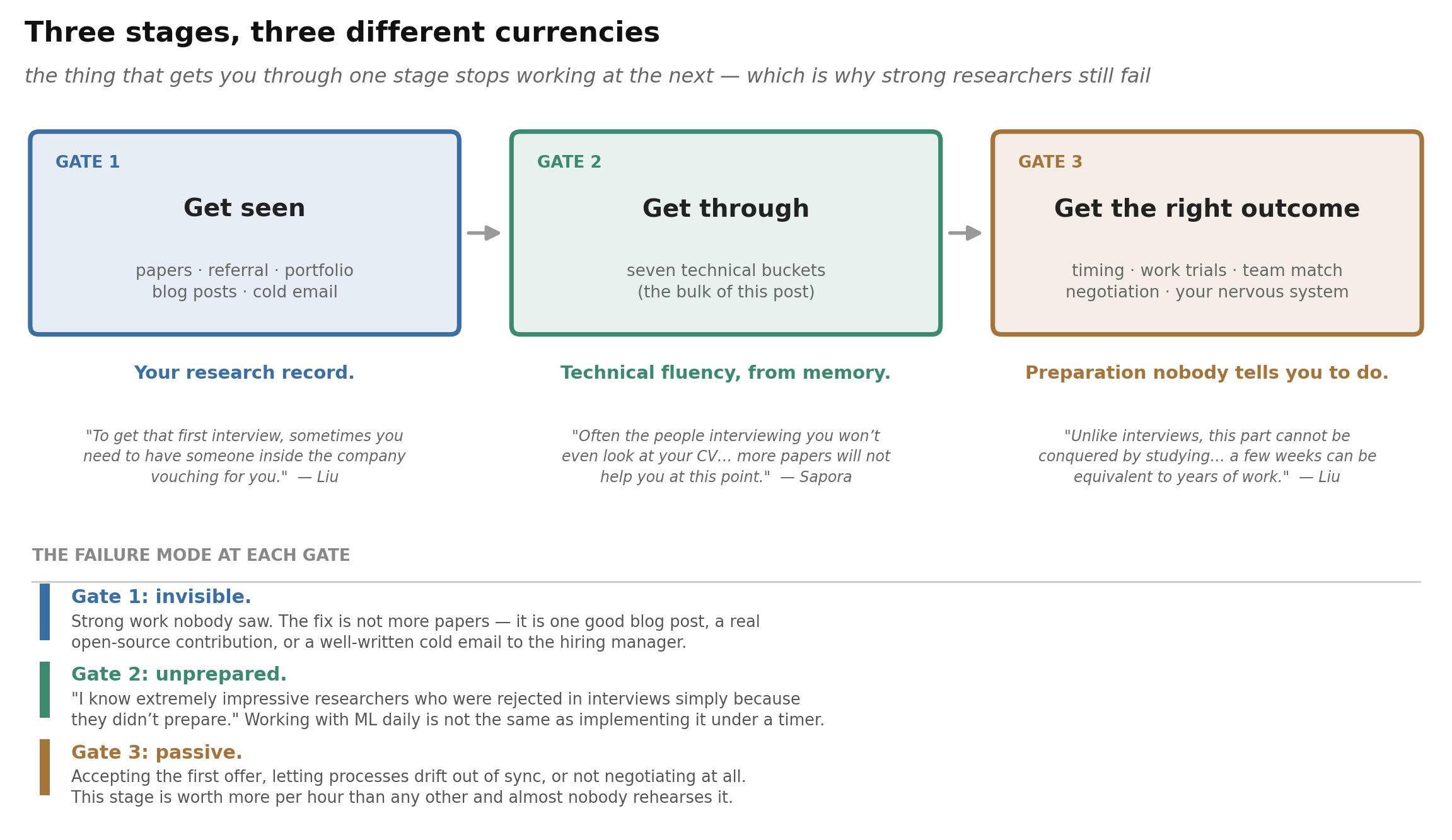 Figure 1. Your research record opens the door and then stops mattering. Technical fluency gets you through the loop and has nothing to do with what you publish. And what you actually walk away with is decided by a third thing that nobody tells you to prepare for at all.
Gate 2 — the technical loop — is where most preparation effort goes, and most of this post is about it, because it is the part with the most learnable content. But it is worth being honest up front that it is the middle third of the problem, not the whole of it.
Inside gate 2 there is a second structural fact. When every round probes hands-on depth in a different part of the stack, every round becomes a veto. The loop scores your minimum, not your maximum.
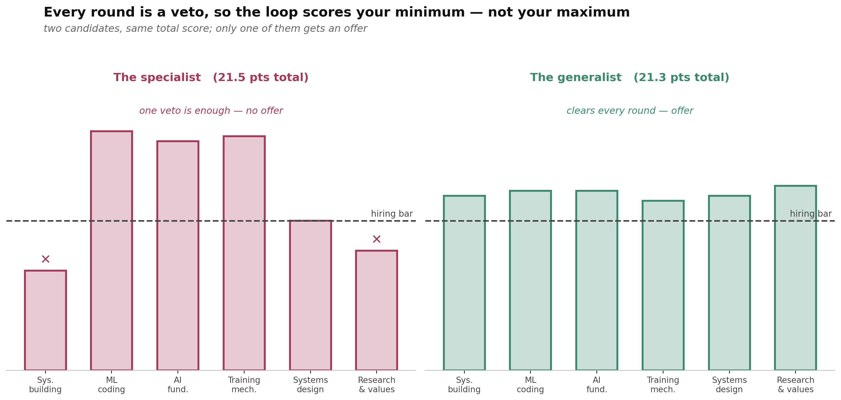 Figure 2. Conjunctive scoring. Being exceptional at four things and weak at one is usually worse than being solidly good at seven, even though the totals are identical.
And the weak spot is rarely random. It is almost always the bucket you decided didn’t apply to you. Yuan Meng, an ML engineer with offers from nearly every lab she onsited at, says her worst round is object-oriented system building — the “just SDE coding” bucket ML people write off [34]. Mimansa Jaiswal, preparing for research roles, hit her ceiling on RLHF — the bucket a researcher assumes they own [21]. Sapora’s warning is the sharpest version:
“I know extremely impressive researchers who were rejected in interviews simply because they didn’t prepare. Working with ML day in and day out is not the same as being ready to implement attention from scratch, derive the backward pass, or code flash attention.” [42]
So, the thesis:
A frontier-lab loop is three tests wearing one name. Your research record gets you seen. Technical fluency — the kind you can produce from memory under a timer — gets you through. And a third body of unglamorous work, around timing and negotiation and your own nervous system, decides what you actually end up with. Optimizing only the middle one is the standard mistake.
Within the technical middle, the common plan has four parts: general coding (usually discounted), ML coding, AI fundamentals, and training mechanisms. That plan misses three of the seven things being scored and mischaracterizes a fourth.
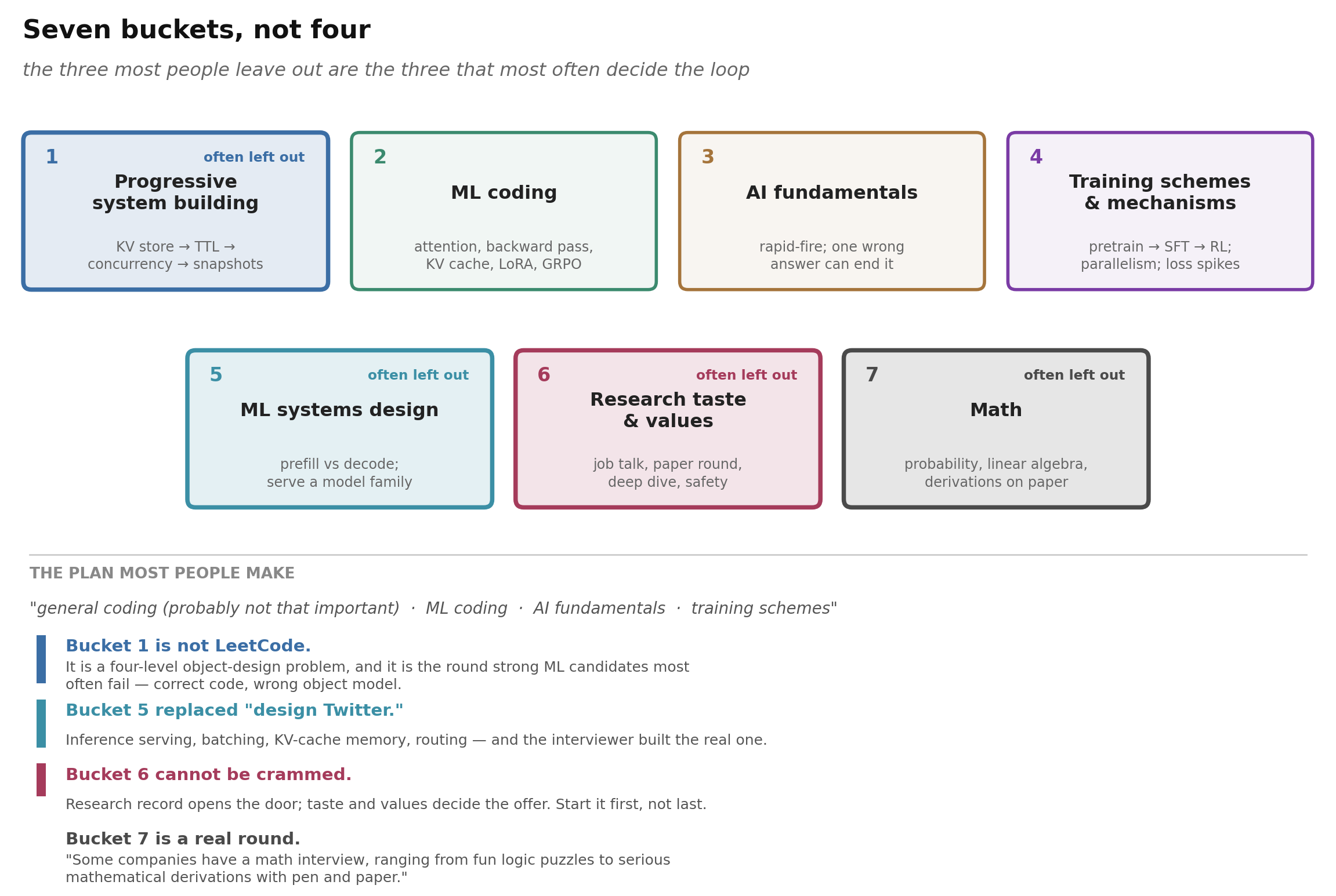 Figure 3. Bucket 1 is not LeetCode. Bucket 5 replaced classical system design. Bucket 6 cannot be crammed. And bucket 7 — a dedicated math round — is real, and is the one I had never seen written down until Liu listed it.
The rest of this is one section per gate, and one per bucket. It is long on purpose: the point is to be something you work through, not something you skim.
Where this comes from
A warning, because this topic has a pollution problem.
Search for any of this and you will drown in content farms — sites selling a course or a tool, all reporting the same specific-sounding numbers. Those numbers agree with each other suspiciously well, which is evidence of cross-generation rather than corroboration. I am not repeating any of them. If you have seen “you need 520 out of 600 on the CodeSignal,” “the acceptance rate is under 1%,” or a precise compensation ceiling, I could not trace any of it to a primary source, so none of it appears below as fact.
I will also admit a research failure that shaped an earlier version of this post. I first went looking for interview questions, and found the second tier: Meng [34] and Jaiswal [21], both genuinely useful. The four accounts this post is actually built on are job-search narratives, which is a different genre that ranks differently, and I missed them on the first pass. They are:
- Alisa Liu [30] — PhD → OpenAI. 11 companies, 57 interviews, 46 recruiter calls, 16 post-offer chats. The most complete taxonomy of round types anywhere, and the best writing on negotiation.
- Silvia Sapora [42] — PhD → DeepMind. Offers from every company whose process she finished. The best concrete target list for what to be able to implement, and unusually honest about the emotional cost.
- Yong Zheng-Xin [55] — PhD, pivoted into safety mid-search. Written explicitly as a complement to the other two; his contribution is six ways the process surprised him, most of which contradict the tidy version.
- Nathan Lambert [26][27] — the only source written from the hiring chair, plus his own 2022 PhD job hunt, which is where the practice of publishing these timelines seems to have started.
One lab-official document exists and is worth reading in full: Anthropic’s guidance on candidate AI usage [2]. Its core instruction is unambiguous — prepare with Claude all you like, but in live interviews “This is all you–no AI assistance unless we indicate otherwise.”
For structure and volume I also use Alexey Grigorev’s AI Engineering Field Guide [13], the only data-driven resource I found: 4,894 job descriptions, per-company interview data for 51 companies, and every question in its bank footnoted to where it was reported.
On X. Several widely-shared threads circulate on this topic; X now requires login to read them, so I have not quoted text I could not read. Where a thread points at a public artifact — Gauri Gupta’s optimization notes [14], Grigorev’s repository — I went to the artifact and cited that instead.
And the caveat that applies to all of it, from Yong: the rounds are far less standardized than any guide implies. He was asked system design, asyncio concurrency, and had rounds evaluating how well he drives AI agents. “always expect wildcard questions and diverse interview rounds” [55]. Treat everything below as a prior, and replace it with what your recruiter actually tells you.
Two running examples
Two objects recur throughout.
E1 — causal self-attention. It appears first as a 25-minute coding prompt, then returns as a fundamentals question, a mechanism question, a systems-design question, and a research question. Same object every time, which is the point.
E2 — a 100B-parameter pretraining run that spikes at step 42,000. Enters as a debugging question and reappears wherever training infrastructure does.
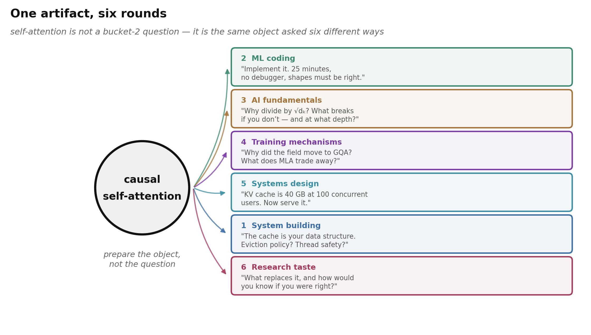 Figure 4. Prepare the object, not the question. Knowing self-attention six levels deep partially prepares you for six different rounds.
Takeaway. Three gates, not one. Prepare for the union of the buckets in the middle gate, and do not let the first and third go unprepared just because nobody frames them as tests.
Gate 1: getting seen
Before anyone can evaluate you, someone has to decide to talk to you. This stage has the widest funnel, the longest lead time, and — going by the four accounts — the least deliberate effort from most candidates.
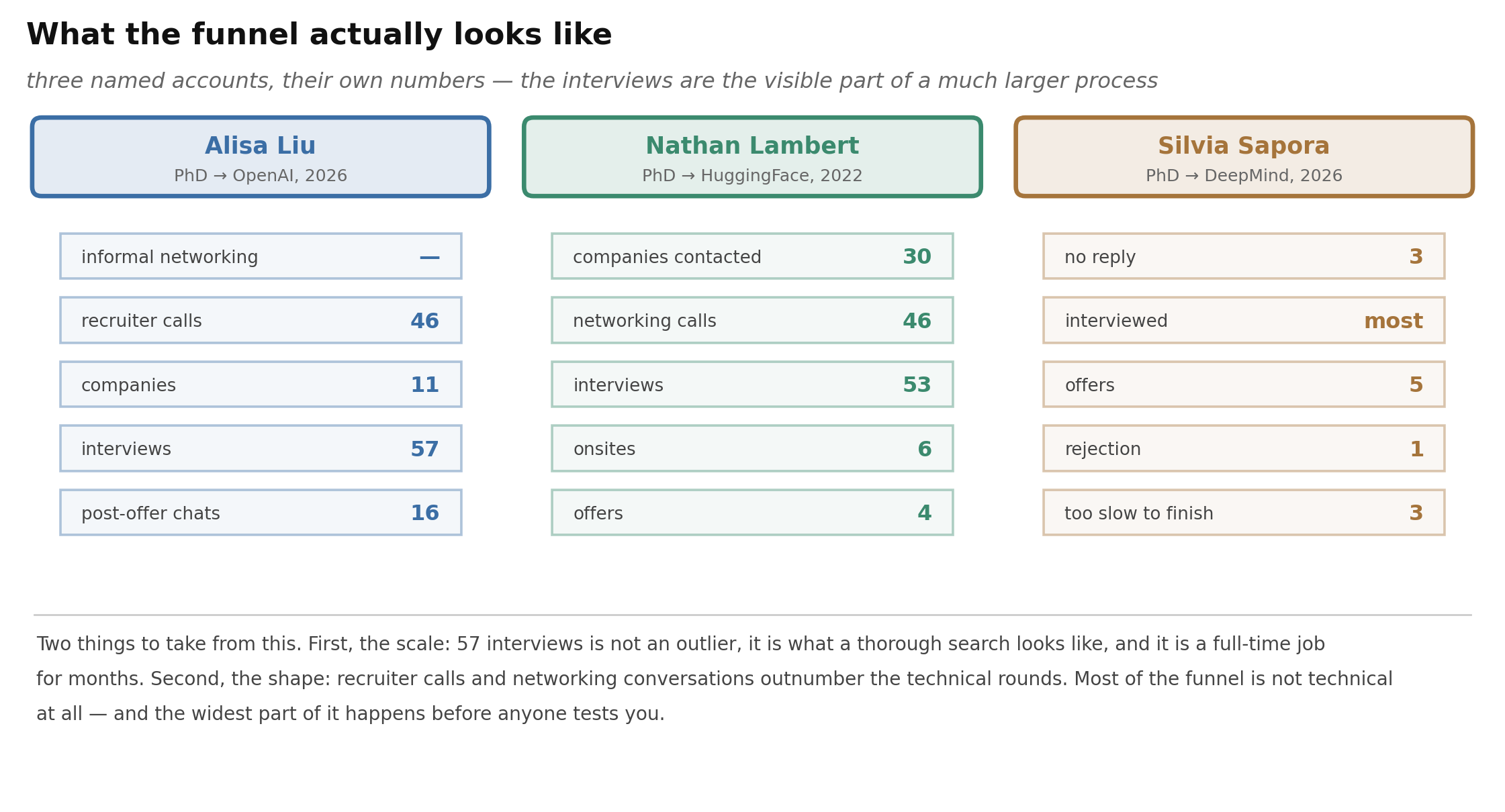 Figure 5. Three named accounts with their own numbers. Note the shape: recruiter calls and networking conversations outnumber technical rounds in every case. Most of the funnel is not technical, and the widest part of it happens before anyone tests you.
Two things to take from that figure. The scale is larger than people expect — 57 interviews is not an outlier, it is what a thorough search looks like, and Liu is explicit that “the job search is a full-time job” [30]. And the composition is not what you would guess: Liu logged 46 recruiter calls on top of 57 interviews; Lambert logged 46 networking calls against ~53 interviews [26].
What actually produces a first interview
The honest answer from the candidate side is: a person. Liu:
“To state the obvious: try to do good work during the PhD, make friends, and collaborate a lot! To get that first interview, sometimes you need to have someone inside the company vouching for you. You can set yourself up for success early on by being social at conferences, collaborating widely, and attending networking events (of course this part doesn’t come easily to everyone — certainly not for me — so take care of your own energy and comfort levels too).” [30]
That last parenthesis matters. Neither she nor Lambert describes this as natural or comfortable. Liu frames the reconnecting part generously: “a big part of the job search is reconnecting with people who you may not have talked to in years — this is okay, expected, and turns out to be a wonderful side effect of the process” [30].
Sapora gives the only explicit CV benchmark I found, and immediately undercuts its importance: “3+ first-author papers and at least one internship or industry role seems to be the threshold for consistently getting callbacks at top labs” — followed by the instruction to stop working on papers once interviews start arriving [42]. Her own experience shows the noise in the process: she got interviews at almost everywhere she applied, and complete silence from three companies (Waymo, Wayve, SpaceXAI) with no discernible reason.
Referrals are worth having and not worth agonizing over. Sapora had a referral for two DeepMind roles and none for a third, and “got invited to interview for one referred role and the unreferred one” [42]. At Anthropic she heard nothing until an ex-colleague referred her. Meng takes the opposite view and skipped referrals entirely, on the theory that a strong profile converts anyway and a referral for a bad fit just produces a faster rejection [34]. Both can be true; the cost is low.
Signals, and the ones that count against you
This is where Lambert’s hiring-side perspective is worth more than any candidate account, because he is describing what he actually does with an application.
“It’s been said that you can tell someone is a genius by reading one Tweet from them, and I agree with this. The written word is still an incredibly effective and underutilized communication form. One excellent blog post can signify real, rare understanding. The opposite holds true for AI slop. One AI slop blog post will kill your application.” [27]
That is an asymmetric bet worth understanding: writing publicly has a high ceiling and a real floor. Publishing something thoughtful is one of the highest-leverage things you can do; publishing model-generated filler is actively negative.
He also names a negative signal I have not seen written down anywhere else: “A small but clear negative signal is a junior researcher being a middle author on too many papers. Just say no, it helps you” [27]. The underlying principle is depth before breadth — “Too many early career researchers try to build breadth of impact (e.g. collecting contributions on many projects) before clearly demonstrating, to themselves and their advisors, depth.”
On open source, he is positive but realistic. It converts more often than open research groups in his experience, but it is getting harder: “standing out amid the sea of AI slop PRs and Issues will be hard. That’ll take class, creativity, humanity, and patience” [27]. Gordić’s older argument for portfolio-over-credentials still holds and is stated more warmly: he would rather hire someone whose work he has watched over months in an open-source project than someone he tested for five hours [11].
Two other channels Lambert names that are easy to overlook: “Some companies hire heavily out of Twitter, some hire from communities such as GPU Mode or NanoGPT speedrunning” [27].
And the frame he applies at the end, which is the most useful thing to keep in mind when you are tempted to over-sell yourself: “The first question to ask is ‘is this person good?’ The second question is, ‘will this person thrive here?’” [27]
Cold emails
Both sides of the table endorse these, and Lambert explains the failure mode precisely:
“Many people you look up to in AI read their emails, the reason you don’t get a response is because you didn’t format your email correctly. The best cold emails show the recipient that they learned from it or obviously benefitted from getting it. Platitudes and compliments are of course nice to receive, but the best cold emails inspire action.” [27]
Two of his recent hires came in through this side door rather than the careers page. Sapora emailed her DeepMind hiring manager and got a reply; her advice is not to restate your CV but to “explain why you’d be a good fit for that specific team and what genuinely excites you about their work” [42]. Her single biggest regret is not doing this more: “Be more proactive about the companies that ignored me… If you really want to work somewhere and you’re not hearing back, do something about it” [42].
One small note on cover letters, from Sapora, since the temptation is obvious: “Please, for the love of everything I hold dear, do not just ask Claude / Gemini / ChatGPT to write it for you. You can absolutely write it yourself and then ask one of them to polish it, that’s fine” [42]. This is also exactly what Anthropic’s own candidate guidance asks for — draft it yourself, then refine [2].
Takeaway. This gate runs on a clock measured in years, not weeks. One good public artifact, a few real relationships, and a well-written email to a specific person will do more than another paper.
The shape of the loop
Before planning a single hour of study, get the round list. Meng’s rule:
“I only start preparing after having several phone screens lined up, since different companies have different interview loops — I don’t know how to start before recruiters explain what the interview rounds are and what each round entails.” [34]
The obvious objection is that it is too late by then. Her answer: you control when the loop starts after the recruiter call, and “if a company isn’t hiring for at least 2–3 months, why would you want to join them?” [34] Lambert adds a concrete version from the other side — ask the recruiter what to prepare, and “sometimes the recruiter actually will give you a topic area like threading or object oriented programing” [26].
Liu’s taxonomy is the most complete, and I use her categories rather than the ones the guides use [30]:
| Round | What it is | Frequency, per Liu |
|---|---|---|
| ML coding | Implement an architecture, a decoding strategy, an ML algorithm, “or sometimes way more creative things” | “by far the most common” |
| General coding | LeetCode, sometimes with flavour | Common |
| Technical discussion (deep) | Design experiments to answer a research question; defend choices; interpret hypothetical results | Common |
| Technical discussion (rapid-fire) | Breadth check. Her examples: “What are some different ways of encoding positional information? What is 5D parallelism? What is the difference between PPO and GRPO?” | Common |
| Research discussion | A past project, then wherever it flows | Common for research roles |
| Behavioral | Textbook, plus the occasional AI-safety question | Universal |
| Math | “fun logic puzzles to serious mathematical derivations with pen and paper” | Some companies |
| Job talk | Shorter than academic, focused on one paper or direction | Research roles |
Note the split in technical discussion, because it changes how you prepare: “The former type of interview tests how you think, whereas the latter checks your breadth of knowledge on the field” [30]. You cannot cram the first and you cannot reason your way through the second.
Sapora’s count for the technical portion: 3 to 8 interviews depending on the company [42].
Three structural points that generalize better than any specific cell:
The rounds are less standardized than they look. This is Yong’s central correction, and it is worth taking seriously precisely because it is inconvenient. He got system design, parallel programming with asyncio, and rounds assessing how he uses AI agents [55]. Meta has an AI-enabled coding round where you debug an unfamiliar multi-file codebase with an LLM available [34]. Anthropic’s live rounds are explicitly AI-free [2]. Ask which one you are in.
A lot of it will have nothing to do with your specialty. Yong pivoted into AI safety and expected safety-heavy interviews; instead, “it still felt like I was evaluated on how well-rounded an AI researcher I was” [55].
References and team matching are separate gates at the end. Meng notes all frontier labs she encountered asked for two to three references pre-offer [34] — a preparation item with a multi-year lead time. And clearing the technical bar does not mean you have a job: when only a couple of teams have headcount, “your years of experience, project complexity, and interview performance are evaluated all over again” [34]. Yong adds that return offers are rare for research roles, unlike SWE; he went through OpenAI’s full loop despite having been an Astra Fellow there [55].
Takeaway. Ask for the exact round list and the passing criteria, then prepare for the loop you actually have — while budgeting for at least one round that nobody warned you about.
Bucket 1: Progressive system building
This is the round people mean when they say “the coding round is not LeetCode,” and it is the one most often underestimated by ML candidates.
The format is a single problem with levels that build on each other, typically 45 to 90 minutes. You implement a small system, then extend it three times as new requirements arrive. The Field Guide’s framing is the clearest I have seen: “code must be extensible since each level builds on prior code” [13]. Reported instances include building an in-memory key-value database starting from SET/GET/ DELETE, implementing a web crawler, a credits-management system with escalating expiry and usage rules, an in-memory database with SQL-like operations, and — memorably — refactoring 100 to 120 lines of convoluted, deeply nested code [13].
Meng’s list of problems in this family: time-based key-value store, in-memory database, a C-like memory allocator, a type inference engine, a circuit breaker, an API gateway with rate limiting, LRU/LFU cache, thread pool / task scheduler, transaction or credit system [34].
Notice what these have in common. They are all miniature versions of real backend infrastructure. None of them has a clever trick. All of them have an object model that is either right or wrong.
The four-level ladder
The escalation is predictable enough to prepare for directly:
| Level | What is added | What is actually being tested |
|---|---|---|
| 1 | Core functionality, single-threaded, minimal API | Can you pick the right data structures and get something working fast? |
| 2 | Constraints, edge cases, more API surface | Did your level-1 design leave room, or must you rewrite? |
| 3 | Concurrency, performance guarantees, correctness under contention | Do you understand shared mutable state? |
| 4 | Extensibility, pluggability, configuration, failure handling | Would this survive contact with production? |
Level 3 is where ML candidates fall off, because it is the one level that has nothing to do with algorithms. It is also, in one candidate’s account of an Anthropic screen, flagged by the recruiter in advance: you should be familiar with handling parallelism. (That one comes from a forum compilation rather than a named author, so treat it as a rumour with a plausible shape — but a cheap one to act on.)
Worked example: a key-value store, four times
Let me take the most commonly reported prompt all the way through, because the decisions are the content, not the code.
Level 1 — set, get, delete.
The naive answer is a dict. The naive answer is correct. Do not over-engineer level 1; you need the time later. But say out loud why you’re choosing what you’re choosing, because the interviewer is already forming a view of whether you think in interfaces.
class KVStore:
    def __init__(self):
        self._data: dict[str, bytes] = {}

    def set(self, key: str, value: bytes) -> None:
        self._data[key] = value

    def get(self, key: str) -> bytes | None:
        return self._data.get(key)

    def delete(self, key: str) -> bool:
        return self._data.pop(key, None) is not None
The one decision worth flagging aloud: delete returns whether something was removed rather than raising. Idempotent deletes are what a real client wants, and saying so costs four seconds.
Level 2 — add TTL.
Here is where the round starts sorting people. The obvious implementation stores an expiry alongside each value and checks it on read. The obvious implementation has a bug that interviewers watch for specifically: a candidate racing to level 4 forgets to check TTL on read, so expired keys stay visible until something else touches them.
The subtler design question is lazy versus active expiry. Lazy expiry (check on access) is trivial but leaks memory for keys that are never read again. Active expiry (a background sweeper) reclaims memory but costs a thread and introduces its own concurrency problems. The right answer in an interview is usually “lazy by default, with an optional sweeper,” and the reason to say that is that it is what Redis does.
import time
from dataclasses import dataclass


@dataclass(slots=True)
class _Entry:
    value: bytes
    expires_at: float | None  # monotonic seconds; None means no expiry


class KVStore:
    def __init__(self, clock=time.monotonic):
        self._data: dict[str, _Entry] = {}
        self._clock = clock  # injected so tests do not have to sleep

    def _live(self, key: str) -> _Entry | None:
        entry = self._data.get(key)
        if entry is None:
            return None
        if entry.expires_at is not None and entry.expires_at <= self._clock():
            del self._data[key]  # lazy expiry: reclaim on the read that noticed
            return None
        return entry

    def set(self, key: str, value: bytes, ttl: float | None = None) -> None:
        expires_at = None if ttl is None else self._clock() + ttl
        self._data[key] = _Entry(value, expires_at)

    def get(self, key: str) -> bytes | None:
        entry = self._live(key)
        return None if entry is None else entry.value

    def delete(self, key: str) -> bool:
        existed = self._live(key) is not None
        self._data.pop(key, None)
        return existed
Two things here are worth more than the code. First, injecting the clock — it signals that you think about testability without being asked, and it means the interviewer’s follow-up (“how would you test expiry?”) is already answered. Second, routing every read through _live means TTL cannot be forgotten at any future level. That is what “extensible” means in practice: the invariant lives in one place.
Level 3 — make it thread-safe.
The reflex is to wrap everything in one lock. That is correct and you should do it first, because a correct coarse lock beats a subtly broken fine-grained one. Then, having done it, say what you’d do next.
import threading


class KVStore:
    def __init__(self, clock=time.monotonic, shards: int = 16):
        # sharding: independent locks so unrelated keys do not contend
        self._shards = [({}, threading.RLock()) for _ in range(shards)]
        self._clock = clock

    def _shard(self, key: str):
        return self._shards[hash(key) % len(self._shards)]

    def set(self, key: str, value: bytes, ttl: float | None = None) -> None:
        data, lock = self._shard(key)
        expires_at = None if ttl is None else self._clock() + ttl
        with lock:
            data[key] = _Entry(value, expires_at)

    def get(self, key: str) -> bytes | None:
        data, lock = self._shard(key)
        with lock:
            entry = data.get(key)
            if entry is None:
                return None
            if entry.expires_at is not None and entry.expires_at <= self._clock():
                del data[key]
                return None
            return entry.value

    def compare_and_set(self, key: str, expected: bytes | None, value: bytes) -> bool:
        """The primitive that makes concurrent clients composable."""
        data, lock = self._shard(key)
        with lock:
            current = data.get(key)
            if (current.value if current else None) != expected:
                return False
            data[key] = _Entry(value, None)
            return True
The things that earn credit at this level, roughly in order:
- Naming the race before you fix it. “Between the
getthat checks expiry and thedelthat acts on it, another thread can write a fresh value, and we’d delete live data.” Then fix it by moving both inside the lock. - Sharding rather than one global lock, with an explicit statement of the trade-off: throughput improves, but any operation spanning multiple keys now needs either a global lock or an ordered multi-lock acquisition to avoid deadlock.
- Offering
compare_and_set. Read-modify-write from a client is not safe no matter how good your internal locking is; the client needs an atomic primitive. Volunteering this is a strong signal. - Knowing what the GIL does and does not do. In CPython the GIL makes individual dict operations atomic but does not make your check-then-act sequences atomic. Saying this correctly separates people who have debugged concurrent Python from people who have read about it.
Level 4 — persistence, snapshots, eviction.
Level 4 is usually open-ended, and the interviewer is now evaluating judgment more than code. The move is to enumerate the axes, state a default, and ask which one they want:
- Durability. Append-only log of mutations plus periodic snapshot compaction (this is Redis AOF plus RDB, and saying so is free credit). Discuss whether the write is acknowledged before or after fsync — that is the actual durability/latency knob.
- Eviction under a memory bound. LRU needs a hash map plus a doubly linked list for O(1); LFU needs frequency buckets. Say which one fits the access pattern rather than defaulting to LRU by reflex.
- Snapshot isolation. A reader iterating the store while writers mutate it needs either copy-on-write or a version counter per entry. This is the level-4 question most likely to be asked as “what if I want to back it up without stopping writes?”
- Failure handling. What happens on a partial write to the log? You need a checksum per record and a truncate-to-last-valid-record recovery path.
Why strong ML candidates fail this round
Meng’s self-diagnosis is worth quoting at length because it is the most useful thing anyone has written about this round:
“I used to think it’s the quickly part that got me. Then, in a mock interview with a backend engineer, I came to see the real issue: my code passes test cases and looks clean, but I make ridiculous design choices no good backend engineer would make. For example, when designing a cart, I chose to store price, units, and other attributes directly in an
Itemdata class, whereas a backend engineer may use a uniqueproduct_idand link it to external metadata when needed.” [34]
That is the whole failure mode. The code runs. The tests pass. The object model says you have never maintained a system where the price changes after the order is placed.
Three habits fix most of it:
- Model identity separately from state. Entities get stable IDs; mutable attributes live where they can be updated once, not copied into every reference.
- Put invariants in one place. If TTL is checked in three methods, one of them will eventually be wrong. Route reads through one accessor.
- Assume the next requirement is coming. It is. That’s the format.
The other half of the fix is just exposure. Meng recommends learning the principles rather than collecting problems — “Some folks obsess over collecting problems other candidates have seen in interviews — this is really tiring and risky… What if you see a new problem and new variants of an old problem? You panic and fail” [34]. The Field Guide agrees and adds the drill that actually works: build one project with layers you add incrementally, then “practice extending it under time pressure. If your initial design can’t handle new requirements without rewriting, that’s the signal to redesign” [13].
Question bank
Short answers; the point is the shape of the response, not the word count.
Design a rate limiter. Start by asking which semantics: fixed window (cheap, allows 2× burst at the boundary), sliding window log (exact, memory grows with request count), sliding window counter (interpolates between two fixed windows, good compromise), or token bucket (allows controlled bursts, which is usually what an API actually wants). Default to token bucket and say why: it is O(1) memory per client, it is the only one that expresses “sustained rate plus burst allowance” naturally, and it is what most production gateways implement. Then the distributed follow-up: the counter has to move to Redis, the check-and-decrement has to be atomic (Lua script or INCR with expiry), and you must decide whether you tolerate slight over-admission during a partition.
Design an LRU cache with O(1) operations. Hash map from key to node, plus a doubly linked list with sentinel head and tail nodes. The sentinels are the part people fumble — they remove every null check from the splice logic. On get, move the node to the front. On put past capacity, evict from the tail. Follow-up: make it thread-safe (one lock is fine; explain why lock-free is hard here), then make it LFU (frequency buckets, each an LRU list, plus a pointer to the minimum frequency).
Implement a circuit breaker. Three states: closed, open, half-open. Closed counts failures in a rolling window; crossing the threshold trips it to open. Open rejects immediately and starts a cooldown timer. After cooldown, half-open lets a limited number of trial requests through; success closes it, failure re-opens it with (ideally) a longer cooldown. The subtlety worth raising: in half-open you must limit concurrency, or a burst of queued requests all get through at once and hammer a service that is still sick.
File deduplication over files too large to fit in memory. Reported in candidate accounts, and it is not really a hash-table question. Stream in fixed-size chunks; hash each chunk; compare hashes rather than content. Then the real discussion: fixed-size chunking breaks under insertion (everything shifts), so content-defined chunking with a rolling hash gives you shift-resistant boundaries. Then: how do you keep the hash index itself from exceeding memory? Shard by hash prefix and spill to disk. Then: what is your collision policy — do you verify bytes on a hash match, or accept the birthday-bound risk with a 256-bit hash?
Design a web crawler. Reported at Anthropic [13]. Single-threaded first: a frontier queue, a visited set, a fetch-parse-enqueue loop. Then politeness (per-domain rate limits and robots.txt), which forces the frontier to become per-domain queues rather than one global queue. Then concurrency (a worker pool with a shared frontier, which raises the visited-set race). Then distribution (partition the URL space by domain hash so politeness stays local to one worker; a Bloom filter for the visited set once it outgrows memory). Then the failure cases: traps, redirect loops, duplicate content under different URLs.
Time-based key-value store. set(key, value, timestamp) and get(key, timestamp) returning the value at the largest timestamp ≤ the query. Per-key list of (timestamp, value) with binary search on read. The follow-up is almost always: what if timestamps arrive out of order? Then you need insertion into a sorted structure, and you should discuss whether you pay on write (keep sorted) or on read (sort lazily).
Takeaway. Three clean levels beat four broken ones. The person grading you is a backend engineer, and they are reading your object model, not your algorithm.
Bucket 2: ML coding
This is the round that has changed most in the last two years, and the one where the gap between “I understand this” and “I can produce this” is widest.
The constraint that defines the round
Everything about how you should prepare follows from one number, which Jaiswal states plainly:
“While these concepts can be coded given sufficient time and debugging capabilities, interview settings present unique challenges. You’ll typically have just 25-35 minutes, need flawless execution, and must maintain precise matrix dimensions throughout.” [21]
Twenty-five minutes, no debugger, shapes must be right. That budget rules out understanding-in-the-moment. Meng puts the same point from the other side:
“In ML coding interviews, you’re expected to write PyTorch as fluently as regular Python. Even if you can Google, you’re bound to run out of time if you need to Google much.” [34]
Her description of the target state: fluent enough to write “MLP, CNN, RNN, Transformer encoders/decoders” and the building blocks — “linear layers, projections, residual connections, layer norm, batch norm, causal self-attention, bidirectional self-attention, activation functions, optimizers” — from memory [34].
There is one habit that pays for itself more than any other, and it comes from Jaiswal:
“Make sure to include dimensions in your variable names or comments. This helps with debugging, and interviewers frequently check dimensions to test your understanding—not just your ability to memorize.” [21]
She later moved from comments to Noam Shazeer’s shape-suffix convention and called it “perhaps even superior” [21]. The idea is to encode the shape into the name: x_BTC for a (batch, time, channel) tensor, q_BHTD after the head split. In a round where the failure mode is a silent transpose, having the shape in the identifier means the bug is visible at the call site rather than three lines later.
Everything below is drawn from a single file that runs as a test suite against PyTorch ground truth, so none of it is code that merely looks right.
  pass   causal MHA matches F.scaled_dot_product_attention
  pass   causal mask actually blocks the future
  pass   KV-cached incremental decode == full recompute
  pass   RoPE attention logits depend only on relative offset
  pass   online (streaming) softmax == naive softmax
  pass   LoRA is identity at init, and merging preserves outputs
  pass   cross entropy matches F.cross_entropy, including ignore_index
  pass   MoE routing respects capacity; aux loss is minimised by a uniform router
  pass   GRPO: zero advantage spread -> ~zero loss; k3 KL is non-negative
  pass   micrograd-style autograd matches torch.autograd, incl. reused nodes
  ...
16/16 checks passed
Attention, and the four traps inside it
Here is E1 — the mechanism from Vaswani et al. [52], in the version you should be able to produce without thinking.
import math
import torch
import torch.nn as nn
import torch.nn.functional as F


class CausalSelfAttention(nn.Module):
    def __init__(self, d_model, n_heads, max_len=512, dropout=0.0):
        super().__init__()
        assert d_model % n_heads == 0, "d_model must be divisible by n_heads"
        self.n_heads = n_heads
        self.d_head = d_model // n_heads
        self.qkv = nn.Linear(d_model, 3 * d_model, bias=False)
        self.proj = nn.Linear(d_model, d_model, bias=False)
        self.attn_drop = nn.Dropout(dropout)
        self.resid_drop = nn.Dropout(dropout)
        self.register_buffer(
            "mask", torch.tril(torch.ones(max_len, max_len)).view(1, 1, max_len, max_len)
        )

    def forward(self, x):
        B, T, C = x.shape
        q, k, v = self.qkv(x).split(C, dim=2)
        q = q.view(B, T, self.n_heads, self.d_head).transpose(1, 2)
        k = k.view(B, T, self.n_heads, self.d_head).transpose(1, 2)
        v = v.view(B, T, self.n_heads, self.d_head).transpose(1, 2)

        att = (q @ k.transpose(-2, -1)) / math.sqrt(self.d_head)
        att = att.masked_fill(self.mask[:, :, :T, :T] == 0, float("-inf"))
        att = self.attn_drop(F.softmax(att, dim=-1))

        y = att @ v
        y = y.transpose(1, 2).contiguous().view(B, T, C)
        return self.resid_drop(self.proj(y))
Roughly twenty lines. Four of them are where people lose the round.
Trap 1: .contiguous(). After transpose(1, 2), the tensor is a view with non-contiguous strides. .view() requires contiguous memory and will raise. You can use .reshape() instead, which silently copies when needed — but if the interviewer asks why, “reshape copies if it has to, view doesn’t” is the answer they want, and it tells them you know the difference between a tensor and its storage.
Trap 2: scaling by sqrt(d_head), not sqrt(d_model). The dot product runs over the head dimension, so that is the dimension whose variance you are correcting. Getting this wrong still trains, just worse, which is exactly why it is a good interview question.
Trap 3: masking before softmax with -inf, not multiplying by zero after. Multiplying the probabilities by a 0/1 mask after softmax leaves the masked positions contributing to the denominator, so the surviving weights no longer sum to one. Additive -inf before the softmax makes them exactly zero.
Trap 4: fusing QKV into one projection. Three separate nn.Linear calls are mathematically identical and measurably slower — one GEMM beats three at the same total FLOPs because of launch overhead and memory traffic. Do it the fast way and mention why.
The check that the mask actually works is worth internalizing, because it is also how you’d debug it: perturb the last token and confirm nothing before it moves.
y1 = model(x)
x2 = x.clone(); x2[:, -1, :] += 10.0
y2 = model(x2)
assert torch.allclose(y1[:, :-1], y2[:, :-1])   # the past cannot see the future
assert not torch.allclose(y1[:, -1], y2[:, -1])  # but the present did change
If a causal-masking bug ever reaches training, this is the three-line test that finds it. Saying that out loud is worth as much as the implementation.
The backward pass, by hand
Sapora lists this explicitly in her baseline, and it is the item most people skip because they assume autograd has made it obsolete [42]. It has not: labs ask for it precisely because it separates people who know what the framework is doing from people who know how to call it. Liu confirms the same thing from the other side — NumPy showed up in her loop mainly “when writing the backwards pass from scratch” [30].
The derivation is four lines. Write them down before you write any code, because the code is then transcription:
\[O = PV \;\Rightarrow\; dV = P^\top dO,\quad dP = dO\,V^\top\] \[P = \mathrm{softmax}(S) \;\Rightarrow\; dS = P \odot \big(dP - \textstyle\sum_j (dP \odot P)_j\big)\] \[S = \tfrac{1}{\sqrt{d}} QK^\top \;\Rightarrow\; dQ = \tfrac{1}{\sqrt{d}}\, dS\,K,\quad dK = \tfrac{1}{\sqrt{d}}\, dS^\top Q\]def attention_forward(q, k, v, causal=True):
"""q,k,v: (B, H, T, D). Returns (out, cache) for the manual backward."""
d = q.shape[-1]
scale = 1.0 / math.sqrt(d)
s = (q @ k.transpose(-2, -1)) * scale
if causal:
T = q.shape[-2]
mask = torch.ones(T, T, dtype=torch.bool, device=q.device).tril()
s = s.masked_fill(~mask, float("-inf"))
p = F.softmax(s, dim=-1)
return p @ v, (q, k, v, p, scale)
def attention_backward(d_out, cache):
q, k, v, p, scale = cache
d_v = p.transpose(-2, -1) @ d_out
d_p = d_out @ v.transpose(-2, -1)
# softmax Jacobian, applied row-wise without materialising the (T, T, T) tensor
d_s = p * (d_p - (d_p * p).sum(dim=-1, keepdim=True))
d_q = (d_s @ k) * scale
d_k = (d_s.transpose(-2, -1) @ q) * scale
return d_q, d_k, d_v
The one line worth being able to explain is the softmax Jacobian. For a single row, \(\partial p_i / \partial s_j = p_i(\delta_{ij} - p_j)\), so the full Jacobian is \(\mathrm{diag}(p) - pp^\top\) — a dense \(T \times T\) matrix per row, which would be \(T^3\) to materialise. The expression p * (dP - rowsum(dP * p)) is that matrix-vector product computed without ever forming it. Interviewers ask about this specific step.
Two more things that earn credit. The causal mask needs no special handling in the backward pass, because P is already exactly zero at masked positions and the gradient inherits that. And the reason FlashAttention recomputes attention in the backward pass rather than storing it is visible right here: the backward needs P, which is the \(O(N^2)\) object you were trying not to keep.
The MLP backward is the same exercise with less notation, and it is the other half of Sapora’s baseline:
def mlp_forward(x, W1, b1, W2, b2):
    h = x @ W1 + b1
    a = torch.relu(h)
    return a @ W2 + b2, (x, W1, W2, h, a)


def mlp_backward(d_y, cache):
    x, W1, W2, h, a = cache
    d_W2 = a.transpose(-2, -1) @ d_y
    d_b2 = d_y.sum(dim=0)
    d_a = d_y @ W2.transpose(-2, -1)
    d_h = d_a * (h > 0)                       # ReLU'(h); the subgradient at 0 is taken as 0
    d_W1 = x.transpose(-2, -1) @ d_h
    d_b1 = d_h.sum(dim=0)
    d_x = d_h @ W1.transpose(-2, -1)
    return d_x, d_W1, d_b1, d_W2, d_b2
Both are verified against torch.autograd in the reference file, in float64 so that the comparison is exact rather than approximately exact. Two conventions to have ready when asked: gradients with respect to a weight matrix have the same shape as the weight, which is the check that catches most transpose errors; and bias gradients sum over the batch dimension because the bias is broadcast across it.
The KV cache, and proving it correct
The universal follow-up is “now make generation fast.” The answer is that during autoregressive decoding you recompute the keys and values for every previous token at every step, which is pure waste — so cache them. And once you are caching them, the cache size becomes the binding constraint, which is why the field moved to grouped-query attention. Both changes belong in one implementation.
class GroupedQueryAttention(nn.Module):
    """n_kv_heads < n_heads. n_kv_heads == 1 is MQA; == n_heads is plain MHA."""

    def __init__(self, d_model, n_heads, n_kv_heads):
        super().__init__()
        assert d_model % n_heads == 0
        assert n_heads % n_kv_heads == 0, "n_heads must be divisible by n_kv_heads"
        self.n_heads, self.n_kv_heads = n_heads, n_kv_heads
        self.n_rep = n_heads // n_kv_heads
        self.d_head = d_model // n_heads
        self.wq = nn.Linear(d_model, n_heads * self.d_head, bias=False)
        self.wk = nn.Linear(d_model, n_kv_heads * self.d_head, bias=False)
        self.wv = nn.Linear(d_model, n_kv_heads * self.d_head, bias=False)
        self.wo = nn.Linear(n_heads * self.d_head, d_model, bias=False)

    def forward(self, x, cache=None):
        B, T, _ = x.shape
        q = self.wq(x).view(B, T, self.n_heads, self.d_head).transpose(1, 2)
        k = self.wk(x).view(B, T, self.n_kv_heads, self.d_head).transpose(1, 2)
        v = self.wv(x).view(B, T, self.n_kv_heads, self.d_head).transpose(1, 2)

        if cache is not None:
            if "k" in cache:
                k = torch.cat([cache["k"], k], dim=2)
                v = torch.cat([cache["v"], v], dim=2)
            cache["k"], cache["v"] = k, v

        k = k.repeat_interleave(self.n_rep, dim=1)
        v = v.repeat_interleave(self.n_rep, dim=1)

        T_full = k.shape[2]
        att = (q @ k.transpose(-2, -1)) / math.sqrt(self.d_head)
        # query at absolute position (T_full - T + i) may attend to keys 0..(T_full - T + i)
        causal = torch.ones(T, T_full, dtype=torch.bool, device=x.device).tril(
            diagonal=T_full - T
        )
        att = att.masked_fill(~causal, float("-inf"))
        y = F.softmax(att, dim=-1) @ v
        return self.wo(y.transpose(1, 2).contiguous().view(B, T, -1))
The line that separates a real implementation from a memorized one is the mask. With a cache, your query block does not start at position zero — it starts at T_full - T. A plain tril is wrong here. The diagonal=T_full - T offset is what makes a single-token decode step legal (it may attend to everything) while a multi-token prefill step stays properly causal.
And the correctness property you should state before the interviewer asks: cached incremental decoding must be numerically identical to a full recompute.
full = model(x)                       # teacher forcing, one shot

cache, outs = {}, []
for t in range(T):                    # token by token, with cache
    outs.append(model(x[:, t : t + 1, :], cache=cache))
step = torch.cat(outs, dim=1)

assert torch.allclose(full, step, atol=1e-5)
This test passes in the reference file. If you cannot make it pass, your mask offset is wrong — and this is precisely the bug that ships to production as “the model is fine in eval but degrades during generation.”
Now the arithmetic that motivates GQA in the first place. The KV cache is
\[\text{bytes per token} = 2 \times n_{\text{layers}} \times n_{\text{kv heads}} \times d_{\text{head}} \times \text{bytes per element}\]The 2 is for K and V. Nothing else in the formula is subtle, which is why it is a good whiteboard question: it is pure bookkeeping, and either you have done it or you haven’t.
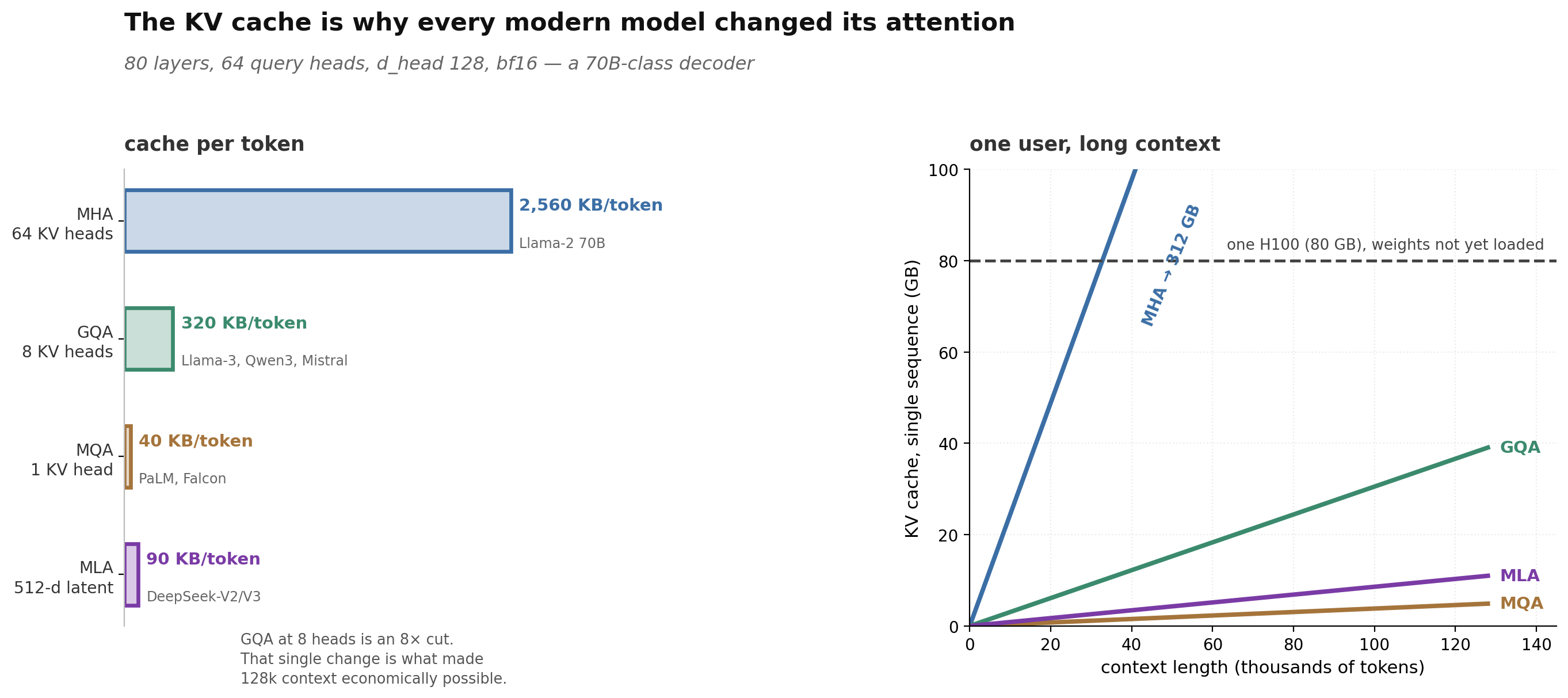 Figure 6. For a 70B-class decoder (80 layers, 64 heads, d_head 128, bf16), plain MHA costs 2.5 MB per token — a single 128k-context conversation would need 312 GB of cache before you load any weights. GQA with 8 KV heads cuts that 8×. This one change is what made long context economically viable.
The variants, and what each trades:
| Variant | KV heads | Bytes/token (above config) | Trade |
|---|---|---|---|
| MHA | 64 | 2,560 KB | Best quality, unaffordable cache |
| GQA [1] | 8 | 320 KB | ~8× cut, quality loss reported as negligible |
| MQA [47] | 1 | 40 KB | 64× cut, measurable quality loss |
| MLA [7] | latent | ~90 KB | Compresses K/V to a low-rank latent; DeepSeek report it beating MHA on quality |
The follow-up worth pre-loading: why did GQA win over MQA? Because MQA’s single shared KV head is too aggressive a bottleneck — quality degrades and training gets less stable — while GQA gives you most of the memory saving with a tunable knob. And why did DeepSeek choose MLA over GQA? Their ablations showed GQA slightly worse than MHA on modeling quality while MLA came out slightly better, which makes MLA the rare optimization that is not a trade-off [7].
Positions: RoPE
Rotary embeddings [51] are asked constantly now, and the reason is that they have a property you can state in one sentence and prove in three lines.
def rope_cache(seq_len, d_head, base=10000.0):
    assert d_head % 2 == 0
    inv_freq = 1.0 / (base ** (torch.arange(0, d_head, 2).float() / d_head))
    t = torch.arange(seq_len).float()
    freqs = torch.outer(t, inv_freq)          # (T, d_head/2)
    return freqs.cos(), freqs.sin()


def apply_rope(x, cos, sin):
    """x: (B, H, T, d_head). Rotates coordinate pairs (2i, 2i+1) by angle m * theta_i."""
    T = x.shape[-2]
    cos, sin = cos[:T], sin[:T]
    x1, x2 = x[..., 0::2], x[..., 1::2]
    rx1 = x1 * cos - x2 * sin
    rx2 = x1 * sin + x2 * cos
    return torch.stack([rx1, rx2], dim=-1).flatten(-2)
The property: RoPE applies an absolute rotation to each of Q and K, but because a dot product between two rotated vectors depends only on the difference of the rotation angles, the resulting attention logit is a function of the relative offset alone. Concretely, positions (5, 2) and (20, 17) give the same logit; (5, 2) and (5, 4) do not. The reference file asserts exactly this.
Three follow-ups that come immediately:
- Where is RoPE applied? To Q and K only, after the head split, before the dot product. Never to V — V carries content, not position.
- Why does RoPE extrapolate poorly past the training context? The low-frequency components complete less than one full rotation during training, so the model never sees those angles and has no basis for interpolating them. This is what position interpolation and NTK-aware / YaRN scaling exist to patch.
- How does RoPE interact with a KV cache? You cache the post-rotation keys. Caching pre-rotation keys and rotating on read would work too, but wastes compute per step.
Online softmax, which is FlashAttention
Interviewers rarely ask you to write a FlashAttention kernel — that is a CUDA exercise. They ask whether you understand the idea, and the idea is entirely expressible in twenty lines of Python.
The problem: the naive attention path materializes an \(N \times N\) score matrix in HBM. At long context that is both the memory ceiling and, because attention is memory-bound, the speed ceiling. FlashAttention [5] avoids it by never materializing the matrix, which requires computing a softmax reduction without having seen all the inputs. That is possible because softmax has a rescaling recurrence:
def online_softmax_weighted_sum(scores, values, block=4):
    """Streaming softmax(scores) @ values without materialising the probability vector."""
    n = scores.shape[0]
    m = torch.tensor(float("-inf"))   # running max
    l = torch.tensor(0.0)             # running denominator
    acc = torch.zeros(values.shape[1])  # running numerator

    for start in range(0, n, block):
        s = scores[start : start + block]
        v = values[start : start + block]
        m_new = torch.maximum(m, s.max())
        correction = torch.exp(m - m_new)   # rescale everything seen so far
        p = torch.exp(s - m_new)
        l = l * correction + p.sum()
        acc = acc * correction + p @ v
        m = m_new
    return acc / l
Every time a block reveals a larger maximum, you rescale the accumulated numerator and denominator by exp(m_old - m_new) and carry on. The result is bit-comparable to a full softmax — the reference file verifies this with deliberately large scores, which is where a naive implementation would overflow.
Sapora’s baseline says “implement flash attention,” and what that means in an interview is the tiled version of the above: an outer loop over query blocks and an inner loop over key blocks, carrying the running statistics per query row.
def flash_attention_forward(q, k, v, block_q=16, block_kv=16, causal=True):
    B, H, T, D = q.shape
    scale = 1.0 / math.sqrt(D)
    out = torch.zeros_like(q)

    for i in range(0, T, block_q):
        qi = q[:, :, i : i + block_q]
        bq = qi.shape[2]
        m = torch.full((B, H, bq), float("-inf"), dtype=q.dtype, device=q.device)
        l = torch.zeros(B, H, bq, dtype=q.dtype, device=q.device)
        acc = torch.zeros(B, H, bq, D, dtype=q.dtype, device=q.device)

        for j in range(0, T, block_kv):
            if causal and j > i + bq - 1:
                break                                   # the whole block is in the future
            kj, vj = k[:, :, j : j + block_kv], v[:, :, j : j + block_kv]
            s = (qi @ kj.transpose(-2, -1)) * scale
            if causal:
                rows = torch.arange(i, i + bq, device=q.device).unsqueeze(1)
                cols = torch.arange(j, j + kj.shape[2], device=q.device).unsqueeze(0)
                s = s.masked_fill(cols > rows, float("-inf"))

            m_new = torch.maximum(m, s.amax(dim=-1))
            correction = torch.exp(m - m_new)
            p = torch.exp(s - m_new.unsqueeze(-1))
            l = l * correction + p.sum(dim=-1)
            acc = acc * correction.unsqueeze(-1) + p @ vj
            m = m_new

        out[:, :, i : i + bq] = acc / l.unsqueeze(-1)
    return out
The reference file has a slightly longer version that also guards the fully-masked-block case, where m stays at -inf and a naive exp(m - m_new) produces nan. That guard is worth mentioning even if you do not write it: it is the bug you hit the moment you run this with a block size that does not divide the sequence length. The tests confirm the output is identical to F.scaled_dot_product_attention and, importantly, independent of block size — which is the property you should offer to verify if the interviewer asks how you would test it.
Say these three things and you have covered the round:
- It is exact, not an approximation. This surprises people and it is the crux of why it was adopted universally.
- Memory goes from \(O(N^2)\) to \(O(N)\); FLOPs actually go up slightly because the backward pass recomputes attention on-chip instead of reading the stored matrix. It is faster anyway, because the operation was bound by HBM traffic rather than by arithmetic.
- The trick is old — the streaming-normalizer recurrence predates the paper [36]. FlashAttention’s contribution is the IO-aware tiling and kernel fusion that makes it win on real hardware.
Sampling, normalization, loss
Three small ones that appear as warm-ups and as “finish the generation loop” follow-ups.
Sampling. The trap is ordering. Temperature must come first (it changes the distribution the truncation acts on), then top-k, then top-p — nucleus sampling, in the original terminology [17].
def sample_next(logits, temperature=1.0, top_k=None, top_p=None, generator=None):
    if temperature == 0:                       # greedy; guard the division
        return int(logits.argmax())
    logits = logits / temperature

    if top_k is not None:
        k = min(top_k, logits.numel())
        kth = torch.topk(logits, k).values[-1]
        logits = logits.masked_fill(logits < kth, float("-inf"))

    if top_p is not None:
        srt, idx = torch.sort(logits, descending=True)
        probs = F.softmax(srt, dim=-1)
        cum = torch.cumsum(probs, dim=-1)
        drop = cum - probs >= top_p            # shift so the crossing token survives
        srt = srt.masked_fill(drop, float("-inf"))
        logits = torch.full_like(logits, float("-inf")).scatter(0, idx, srt)

    return int(torch.multinomial(F.softmax(logits, dim=-1), 1, generator=generator))
The cum - probs >= top_p line is the one to get right: you keep the smallest prefix whose cumulative mass exceeds p, which means the token that crosses the threshold is included, not dropped. Off-by-one here silently changes the sampling distribution. And temperature == 0 needs an explicit branch, because otherwise you divide by zero — a real bug that has shipped in real inference servers.
Cross entropy, which is really a log-sum-exp question:
def cross_entropy(logits, targets, ignore_index=-100):
    keep = targets != ignore_index
    logits, targets = logits[keep], targets[keep]
    m = logits.max(dim=-1, keepdim=True).values
    logsumexp = m.squeeze(-1) + (logits - m).exp().sum(-1).log()
    picked = logits.gather(1, targets.unsqueeze(1)).squeeze(1)
    return (logsumexp - picked).mean()
Subtracting the max before exponentiating is the entire point; without it, logits around 20 overflow in fp32. The ignore_index handling is not decoration — it is how you mask prompt tokens during SFT, so an interviewer asking about instruction tuning may well come back to this function.
RMSNorm, which is what modern models actually use:
class RMSNorm(nn.Module):
    def __init__(self, d, eps=1e-6):
        super().__init__()
        self.weight = nn.Parameter(torch.ones(d))
        self.eps = eps

    def forward(self, x):
        rms = torch.rsqrt(x.pow(2).mean(-1, keepdim=True) + self.eps)
        return (x * rms).type_as(x) * self.weight
No mean subtraction, no bias. The follow-up: why did the field drop LayerNorm’s re-centering? Because ablations showed the re-scaling does the work and the re-centering mostly doesn’t [57], and dropping it removes a reduction over the feature dimension — which matters when you run it twice per layer across 80 layers. Note also the .type_as(x): under bf16 you want the reduction in fp32 and the result cast back, and mentioning that shows you have trained something rather than only read about training.
LoRA
Low-rank adaptation [18] is the one parameter-efficient method everyone is expected to be able to write.
class LoRALinear(nn.Module):
    def __init__(self, base: nn.Linear, r=8, alpha=16, dropout=0.0):
        super().__init__()
        self.base = base
        for p in self.base.parameters():
            p.requires_grad = False
        self.r, self.scaling = r, alpha / r
        self.A = nn.Parameter(torch.zeros(r, base.in_features))
        self.B = nn.Parameter(torch.zeros(base.out_features, r))
        nn.init.kaiming_uniform_(self.A, a=math.sqrt(5))
        # B stays zero: the adapter is an exact no-op at step 0
        self.drop = nn.Dropout(dropout)

    def forward(self, x):
        return self.base(x) + self.drop(x) @ self.A.T @ self.B.T * self.scaling

    @torch.no_grad()
    def merge(self):
        self.base.weight += (self.B @ self.A) * self.scaling
        self.A.zero_(); self.B.zero_()
        return self.base
Two properties the interviewer is checking, both verified in the reference file:
It is the identity at initialization. B starts at zero, so BA = 0 and the adapted model is exactly the base model. If you initialize both matrices randomly, you have silently corrupted your starting point and your first training steps fight to recover. Candidates who initialize both randomly are revealing that they have used LoRA through a library but never read it.
It merges losslessly. \(W + \frac{\alpha}{r}BA\) is just a weight matrix, so after training there is zero inference overhead — unlike adapter layers, which add depth. This is the actual reason LoRA won.
The follow-ups: \(\alpha/r\) exists so you can change rank without retuning the learning rate. Attention projections are the usual target, though adding the MLP matrices helps on harder tasks. QLoRA additionally quantizes the frozen base to 4-bit and keeps the adapter in higher precision, trading a little quality for a lot of memory. And the honest limitation: LoRA is excellent at style, format and task adaptation, and poor at injecting substantial new knowledge — a low-rank update simply does not have the capacity.
Mixture of experts
You will not be asked to write a production MoE layer, but top-1 routing with a capacity limit is a reasonable 20-minute question, and it exposes whether you know why MoE is hard.
def top1_route(logits, capacity):
    """logits: (T, E). Returns (expert_idx, gate, kept_mask) with per-expert capacity."""
    gates = F.softmax(logits, dim=-1)
    gate, expert = gates.max(dim=-1)
    kept = torch.zeros_like(expert, dtype=torch.bool)
    for e in range(logits.shape[1]):
        idx = (expert == e).nonzero(as_tuple=True)[0]
        if idx.numel() == 0:
            continue
        # on overflow, keep the most confident tokens; the rest are dropped
        order = idx[torch.argsort(gate[idx], descending=True)][:capacity]
        kept[order] = True
    return expert, gate, kept


def load_balancing_loss(logits):
    """Switch Transformer aux loss: E * sum_e (fraction routed to e) * (mean prob of e)."""
    gates = F.softmax(logits, dim=-1)
    E = logits.shape[-1]
    expert = gates.argmax(dim=-1)
    frac = torch.bincount(expert, minlength=E).float() / expert.numel()
    prob = gates.mean(dim=0)
    return E * (frac * prob).sum()
The concept the code is there to expose: tokens get dropped. Capacity is finite because the all-to-all communication needs fixed-size buffers, so when a popular expert overflows, the excess tokens skip the layer entirely and pass through on the residual stream. That is the mechanism behind the observation that a batched MoE model can give you slightly different outputs depending on what else is in the batch.
The auxiliary loss is the other half. Routing is a discrete argmax with no gradient, so left alone the router collapses onto a few experts. The Switch Transformer loss [10] multiplies the fraction of tokens routed to each expert by the mean gate probability for that expert, summed and scaled by the expert count. It is minimized at uniform routing, where it equals 1 — the reference file verifies both that a uniform router scores ≈1 and that a skewed router scores higher. Worth mentioning as the current frontier: DeepSeek-V3 dispenses with the auxiliary loss entirely, using a bias term adjusted during training to balance load without adding a gradient that fights the language-modeling objective [8].
Tokenization
Byte-pair encoding [45] comes up more often than people expect, usually as “why does the model count letters badly.”
def bpe_train(text, num_merges):
    ids = list(text.encode("utf-8"))
    merges = {}
    for i in range(num_merges):
        counts = {}
        for pair in zip(ids, ids[1:]):
            counts[pair] = counts.get(pair, 0) + 1
        if not counts:
            break
        best = max(counts, key=counts.get)
        if counts[best] < 2:
            break
        new_id = 256 + i
        merges[best] = new_id
        merged, j = [], 0
        while j < len(ids):
            if j + 1 < len(ids) and (ids[j], ids[j + 1]) == best:
                merged.append(new_id); j += 2
            else:
                merged.append(ids[j]); j += 1
        ids = merged
    return merges
The detail that matters at encode time: merges are applied in the order they were learned, not by frequency in the string being encoded. Getting that backwards produces a tokenizer that round-trips inconsistently, which is a genuinely nasty production bug.
Starting from raw UTF-8 bytes rather than characters is the other decision worth explaining: a byte-level vocabulary can represent any input, so there is no out-of-vocabulary case ever. The cost is that non-Latin scripts consume more tokens per character, which is a real fairness and cost issue and a good thing to raise unprompted.
Autograd
Meng singles this out with visible dread — “how to implement autograd from scratch instead of calling loss.backward()? … Even people who use PyTorch daily rarely know low-level details like how computation graphs are built or how autograd works under the hood” [34]. It is a fair thing to be asked, and it is about forty lines.
class Value:
    """Scalar reverse-mode autodiff, in the spirit of Karpathy's micrograd."""

    def __init__(self, data, _children=(), _op=""):
        self.data = float(data)
        self.grad = 0.0
        self._backward = lambda: None
        self._prev = set(_children)

    def __add__(self, other):
        other = other if isinstance(other, Value) else Value(other)
        out = Value(self.data + other.data, (self, other), "+")

        def _backward():
            self.grad += out.grad      # += , not = : a node may be used many times
            other.grad += out.grad

        out._backward = _backward
        return out

    def __mul__(self, other):
        other = other if isinstance(other, Value) else Value(other)
        out = Value(self.data * other.data, (self, other), "*")

        def _backward():
            self.grad += other.data * out.grad
            other.grad += self.data * out.grad

        out._backward = _backward
        return out

    def backward(self):
        topo, seen = [], set()

        def build(v):
            if v in seen:
                return
            seen.add(v)
            for c in v._prev:
                build(c)
            topo.append(v)

        build(self)
        self.grad = 1.0
        for v in reversed(topo):       # reverse topological order
            v._backward()
Two ideas carry the whole thing, and if you can articulate them you can rebuild the rest under pressure:
Every operation stores a closure that knows how to push gradient to its inputs. The graph is built implicitly by the forward pass; each node captures its parents and its local derivative rule.
Gradients accumulate, and the traversal order is reverse topological. The += is the single most important character in the file — a node used in two places receives gradient from both paths, and = would silently discard one. The topological sort guarantees that when you call a node’s _backward, every consumer of that node has already contributed. The reference file checks this against torch.autograd using an expression where a and b each feed multiple paths, which is precisely the case a naive implementation gets wrong.
Question bank
Beyond what is implemented above, be ready to produce these cold. The list is drawn from what Meng [34], Jaiswal [21] and the Field Guide [13] independently report.
From scratch, in NumPy or PyTorch: an MLP with manual backward; an RNN cell, then LSTM and GRU cells (Jaiswal flags these as the gap in most practice platforms [21]); a 2D convolution with stride and padding; BatchNorm with running statistics, and the train/eval difference; layer normalization; dropout with inverted scaling; Adam from the update rule; a full training loop that overfits ten examples.
Classical ML, still asked: logistic regression with SGD, L2 and early stopping (reported at Mistral [13]); k-means; k-nearest neighbours; a decision-tree split on information gain; PCA via SVD; and the metrics — precision, recall, ROC-AUC, NDCG, MRR — implemented from labels and scores rather than imported.
LLM-specific: beam search with length normalization; greedy decoding with a KV cache; speculative decoding’s accept/reject step; label smoothing; the DPO and GRPO losses (both below, in bucket 4); sliding-window attention; cross-attention for an encoder-decoder.
The debug variant, which is increasingly common: you are handed working-looking model code that trains badly. Have a checklist. Is the loss masked correctly on padding? Is the causal mask off by one? Are the labels shifted relative to the inputs? Is the learning rate sane after warmup? Is the model in train() mode? Are you calling optimizer.zero_grad()? Is dropout active at eval? Is something detaching the graph? Is the data actually shuffled? Meng’s advice for this: overfit a tiny batch first — if the model cannot memorize ten examples, the bug is in the code, not the hyperparameters [34].
Where to drill. The four resources the first-hand accounts converge on, and what each is for: Karpathy’s nanoGPT and micrograd [23] for building a GPT and an autograd engine end to end; Raschka’s Build a Large Language Model (From Scratch) [41], whose repository has separate reference implementations for MHA, GQA, MLA, sliding-window attention, KV caching and MoE — it is the closest thing to a canonical answer key for this bucket; Deep-ML [6], which is LeetCode for ML and is what both Meng and Jaiswal used for volume; and Huyen’s interview book [20] for the fundamentals side. Jaiswal’s trick with book repositories is worth stealing: she turned the notebooks into fill-in-the-blank exercises rather than reading them [21].
Takeaway. Fluency is the deliverable. Reading these implementations is not preparation; typing them from a blank editor, repeatedly, until the shapes come out right the first time, is.
Bucket 3: AI fundamentals
This bucket is dangerous out of proportion to its length. It is often five minutes at the start of a phone screen, and Meng is blunt about the consequences:
“Many candidates are confused when they fail, remembering they’ve solved the coding question perfectly, only to forget that they made fundamental mistakes on ML fundamentals. One or two wrong answers can be enough for rejection.” [34]
The way to prepare is not to memorize definitions. Both anchor sources say the same thing here, and it is worth taking seriously. Meng: “every minute I spend on interview prep should make me a better engineer… Memorizing answers doesn’t do that for me” [34]. Her recommended path is to read Prince’s Understanding Deep Learning [38] — chapters 1–9, 11 and 12 if you’re short on time — and treat the prep as a gap-finding exercise.
The reason memorization fails is structural: the follow-up is always “when does that break?” A definition has no answer to that. So the format below is why is it like that, and each answer carries its own failure mode.
Attention and architecture
Why divide by \(\sqrt{d_k}\)? Take \(q\) and \(k\) with independent components of unit variance. Their dot product is a sum of \(d_k\) such products, so it has variance \(d_k\) and standard deviation \(\sqrt{d_k}\). With \(d_k = 128\) the logits have a spread of ±11 or so before training has done anything. Softmax over logits that wide is nearly a one-hot, and a saturated softmax has vanishing gradients — the attention pattern is frozen at initialization and cannot learn. Dividing restores unit variance. When it breaks: this argument assumes the initialization it describes; with badly scaled inputs or after weights drift, logits can still blow up, which is what QK-normalization was introduced to handle in very large models.
Is there a way to see attention as something familiar? Two framings, both worth having. Murphy’s, via Jaiswal [21]: “We can think of attention as a soft dictionary look up, in which we compare the query \(q\) to each key \(k_i\), and then retrieve the corresponding value \(v_i\).” A hard dictionary returns one value for an exact key match; attention returns a convex combination weighted by similarity. The second, which Meng notes people miss: attention is a soft, learned k-nearest-neighbours. Instead of picking the top-k by a fixed distance metric, it takes a softmax-weighted average over all of them under a learned metric. She points at exactly this as the kind of connection that separates candidates: “we may know KNN and attention well in isolation, but don’t immediately realize how the latter is a softer version of the former” [34].
What does the softmax temperature do? Dividing logits by \(\tau\) before the softmax interpolates between two limits: as \(\tau \to 0\) you get argmax, as \(\tau \to \infty\) you get uniform. It does not change the ranking, only the sharpness. When it matters: at \(\tau\) well below 1 sampling degenerates into repetition loops; above 1 you get incoherence. This is the same knob as the attention scaling, which is a nice thing to point out.
Encoder-only, decoder-only, or encoder-decoder? Encoder-only (BERT) uses bidirectional attention and is trained with masked language modeling — good for classification and retrieval where you embed a fixed input, useless for generation. Decoder-only (GPT) uses causal attention and next-token prediction, which means every position is a training signal and the same model generates. Encoder-decoder (T5) separates the two with cross-attention, which suits genuine sequence-to-sequence tasks like translation. Why did decoder-only win? Training efficiency (every token supervises), architectural simplicity, and the fact that in-context learning turns almost every task into generation.
What is multi-token prediction and why do it? Predicting several future tokens per position, as DeepSeek-V3 does [8], densifies the training signal and gives the model a lookahead objective. It also gives you a free draft model for speculative decoding at inference time.
Normalization, residuals, and depth
Pre-LN or post-LN, and why did the field move? The original Transformer put LayerNorm after the residual add. That places a normalization on the residual path, so gradients get rescaled at every layer and deep models will not train without a carefully tuned warmup. Pre-LN normalizes the input to each sublayer, leaving the residual stream a clean identity path from embedding to output. Xiong et al. [53] showed this is what removes the warmup requirement. The cost: the residual stream’s magnitude grows with depth, so you need a final norm before the output head, and very deep pre-LN models can suffer representation collapse in later layers — which is why variants like sandwich norm exist.
Why LayerNorm and not BatchNorm in transformers? Three reasons, and interviewers want more than one. Sequence lengths vary, so batch statistics are computed over a ragged and inconsistent set of positions. Batch statistics couple examples in a batch, which breaks autoregressive generation with batch size 1 — you would need running statistics that never match training. And in distributed training BatchNorm needs cross-device synchronization on every forward pass. LayerNorm normalizes within a single token’s feature vector, so it is independent of batch composition entirely.
Why residual connections? The usual answer, “they fix vanishing gradients,” is only half of it. The gradient of \(y = x + f(x)\) with respect to \(x\) is \(1 + f'(x)\), so there is always an identity path for gradient to flow along. The better framing is the residual stream view: each layer reads from and writes to a shared bus, so a 100-layer network can behave like an ensemble of shorter paths, and any layer that isn’t useful can learn to write approximately nothing rather than having to learn the identity map [15].
What actually causes exploding gradients in an LLM run, and what do you do? Usually not the depth — pre-LN plus residuals handle that. In practice it is a bad data batch, a learning rate that is too high for the current curvature, or fp16 overflow. Standard mitigations: global gradient-norm clipping (and you should be logging the pre-clip norm, because a spike there is your earliest warning), bf16 instead of fp16, and warmup. If the gradient norm is spiking regularly, clipping is masking a problem rather than solving it.
Optimization
Adam versus AdamW — what does decoupling actually fix? In Adam, L2 regularization is added to the gradient, so it then passes through the same per-parameter adaptive scaling as everything else. The effective weight decay therefore ends up inversely proportional to the gradient’s recent magnitude: parameters with small gradients get decayed hard, parameters with large gradients barely at all. That is not what anyone means by weight decay. AdamW [33] applies the decay directly to the weights, outside the adaptive step, restoring the intended uniform pull toward zero. This is why every modern LLM uses AdamW.
Why does Adam need so much memory, and what can you do about it? Two states per parameter — first and second moment — in fp32. For a model with \(P\) parameters in bf16 you are carrying roughly \(2P\) bytes of weights, \(2P\) of gradients, and \(4P + 4P\) of optimizer state, plus \(4P\) if you keep fp32 master weights: about 16 bytes per parameter before a single activation. That arithmetic is the whole reason ZeRO exists, and being able to produce it on demand is a good signal.
Why warmup? Adam’s second-moment estimate is unreliable in the first few hundred steps, so the adaptive denominator is noisy and the effective step size can be enormous. Warmup keeps you small until the estimate stabilizes. Note the interaction: pre-LN reduces the need for warmup but does not remove the optimizer-state argument for it.
What is muP and why would you care? Standard parameterization makes the optimal learning rate shift as you scale width, so you must re-tune at every size — prohibitive at frontier scale. Maximal update parameterization [54] rescales initialization and learning rates per-layer so that the optimal hyperparameters become width-invariant. You tune on a small proxy model and transfer to the large one. This is a good answer to “how would you choose hyperparameters for a run you can only afford once.”
Anything newer than AdamW? Muon has real traction — it orthogonalizes the momentum update for 2D parameters via a Newton-Schulz iteration, and has been reported to scale to large LLM training with meaningful efficiency gains [32]. Being aware of it signals you read current work; claiming strong opinions about it probably does not.
Scaling and evaluation
Kaplan versus Chinchilla — what changed? Kaplan et al. [22] found power-law scaling in parameters, data and compute, and their analysis suggested that under a fixed compute budget you should spend most of the increase on parameters. Hoffmann et al. [16] revisited it with a better treatment of the learning-rate schedule and found the compute-optimal frontier is roughly equal scaling — about 20 tokens per parameter. That reframed the field: models got smaller and datasets got much bigger.
And what changed again after Chinchilla? Chinchilla optimizes training compute. If you are going to serve a model to millions of users, inference cost dominates total cost, so it is rational to train a smaller model far past its compute-optimal token count — which is what Llama 3 did at ~15T tokens for an 8B model, orders of magnitude past the Chinchilla point [12]. The right answer to “what is the optimal model size” is a question: optimal for training cost, or for total lifetime cost?
Is test-time compute a third scaling axis? Yes, and it has the most interesting shape. Snell et al. [49] showed that under some conditions, spending compute at inference beats spending it on parameters. The practical implication for evaluation is that a single benchmark number is now underspecified — the same weights, run greedily versus with a large search budget, are effectively two different systems.
What is perplexity, and when is it misleading? The exponentiated mean negative log-likelihood per token — the effective branching factor. It is misleading across tokenizers (different vocabularies are not comparable), it is dominated by easy tokens, and after RLHF it typically gets worse while the model gets more useful. Never compare perplexity across models with different tokenizers.
How do you evaluate a model where you cannot check the answer? Say the ladder out loud: exact-match against a verifier where one exists; human preference where it doesn’t; LLM-as-judge as a scalable proxy for the human, with its known failure modes (position bias, length bias, self-preference); and pairwise comparison rather than absolute scoring, because humans and judges are both far more reliable at ranking than at rating. Then the contamination question, which is what a lab actually worries about: how do you know the benchmark isn’t in the training set? N-gram overlap checks, held-out sets built after the training cutoff, and canary strings.
Takeaway. Answer the why, then volunteer the when it breaks. Getting to the failure mode before the interviewer asks is the difference between a correct answer and a good one.
Bucket 4: Training schemes and mechanisms
This is the bucket your framing called “training scheme and mechanism,” and it is the one where the depth gradient is steepest. Almost every candidate can name PPO, GRPO and DPO. Very few can say where the KL term lives in each, and that is exactly the question.
The ladder, and what each rung can fix
Think of post-training as a sequence of distribution shifts, each with a specific job and specific things it cannot do.
| Stage | Data | What it can fix | What it cannot fix |
|---|---|---|---|
| Pretraining | Web-scale unlabeled text | Knowledge, syntax, world model | Following instructions, format |
| Midtraining | Curated high-quality, long-context, code, math | Domain capability, context length | Preferences, style |
| SFT | Demonstrations | Format, instruction-following, tool syntax | Anything not demonstrated; it can only imitate |
| Reward modeling | Preference pairs | A scalar proxy for “better” | Its own misspecification |
| RL | Prompts plus a reward or verifier | Optimizes for the reward, including exploiting it | Knowledge the base model lacks |
| Distillation | Teacher outputs | Cost, latency | Exceeding the teacher, generally |
The single most useful framing to have ready: SFT teaches the model what a good answer looks like; RL teaches it which of its own answers are better. That is why RL keeps working after SFT saturates — SFT can only push toward demonstrations, while RL can rank the model’s own samples and push into regions no human demonstrated. It is also why RL cannot install missing knowledge: it can only reweight what the base model can already produce.
Reward models
The standard reward model is Bradley-Terry. Given preference pairs, you train a scalar head so that
\[\mathcal{L} = -\log \sigma\big(r_\theta(x, y_w) - r_\theta(x, y_l)\big)\]where \(y_w\) is preferred over \(y_l\). Three things to be able to say about it:
The reward is only identified up to a shift. Bradley-Terry constrains differences, not absolute values, so the scale is arbitrary and comparing raw reward values across training runs is meaningless. This is why people normalize rewards per batch.
Reward models are the weak link. They are trained on a narrow distribution of responses and then queried far off it as the policy moves. Overoptimizing against one is the textbook Goodhart case, and it is why the KL penalty exists at all.
Verifiers beat learned rewards where you can get them. A unit test or a math checker is a function, not a neural network, and cannot be hacked in the same way. The causal chain from “this answer is right” to a gradient is much shorter.
PPO, GRPO, DPO: where the KL lives
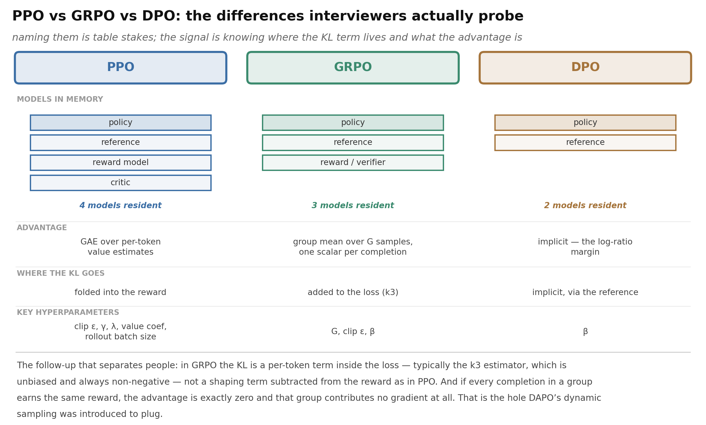 Figure 7. The comparison that interviewers actually probe. Four models resident versus three versus two; per-token GAE versus a group-mean scalar versus an implicit log-ratio; and three different answers to where the KL constraint is applied.
PPO [44] keeps four models in memory: policy, frozen reference, reward model, and a learned critic. The critic exists to reduce variance — without a baseline, the advantage for a sample is its raw reward, and the gradient is dominated by the fact that some prompts are simply easier. Advantages come from GAE [43], which interpolates between high-bias one-step TD and high-variance Monte Carlo:
def compute_gae(rewards, values, gamma=0.99, lam=0.95, last_value=0.0):
    T = len(rewards)
    adv = torch.zeros(T)
    gae = 0.0
    for t in reversed(range(T)):
        next_v = values[t + 1] if t + 1 < T else last_value
        delta = rewards[t] + gamma * next_v - values[t]
        gae = delta + gamma * lam * gae
        adv[t] = gae
    return adv, adv + values
The property to state: \(\lambda = 1\) recovers Monte Carlo (unbiased, high variance) and \(\lambda = 0\) recovers one-step TD (biased, low variance). The reference file asserts both limits, which is also the cheapest way to convince yourself an implementation is right.
The clipped surrogate objective provides a soft trust region — it prevents any single update from moving the policy too far, which is what plain policy gradient lacks. In PPO the KL penalty is conventionally subtracted from the reward before advantages are computed.
GRPO [46] removes the critic. The insight is that the value function is only serving as a baseline, and you can get a baseline for free by sampling a group of \(G\) completions per prompt and using their mean reward.
def grpo_loss(logp, logp_old, logp_ref, rewards, mask,
              clip_eps=0.2, beta=0.04, group_size=None):
    """logp/logp_old/logp_ref: (B, L). rewards: (B,). mask: (B, L) over completion tokens."""
    B = rewards.shape[0]
    g = group_size or B
    r = rewards.view(-1, g)
    adv = (r - r.mean(dim=1, keepdim=True)) / (r.std(dim=1, keepdim=True) + 1e-4)
    adv = adv.reshape(B, 1)                       # one scalar per completion, broadcast over L

    ratio = (logp - logp_old).exp()
    policy = -torch.min(ratio * adv,
                        ratio.clamp(1 - clip_eps, 1 + clip_eps) * adv)

    # k3 estimator: unbiased and always >= 0, unlike a raw log-ratio
    log_ratio = logp_ref - logp
    kl = log_ratio.exp() - log_ratio - 1.0

    return ((policy + beta * kl) * mask).sum() / mask.sum().clamp(min=1.0)
Three details that are the actual interview content:
- The KL moved into the loss, as a per-token term, rather than being folded into the reward. And it is usually the k3 estimator \(e^{-x} + x - 1\) rather than a raw log-ratio, because k3 is unbiased and non-negative — a plain log-ratio difference can go negative sample-to-sample, which is a nonsensical KL estimate.
- The advantage is bandit-style: one scalar per completion, broadcast to every token. There is no per-token credit assignment at all. This is a real limitation and a good thing to name.
- If every completion in a group earns the same reward, the advantage is exactly zero and the group contributes no gradient. The reference file verifies this. On a dataset where most prompts are either always-solved or never-solved, most of your compute produces nothing — which is exactly what DAPO’s dynamic sampling [56] fixes by resampling until a group has reward variance.
DPO [39] skips RL entirely. Its result is that for the KL-constrained RLHF objective, the optimal policy and the reward function are related in closed form, so the reward can be written in terms of the policy itself. Substituting turns preference learning into a classification loss:
def dpo_loss(pi_chosen, pi_rejected, ref_chosen, ref_rejected, beta=0.1):
    """All arguments are summed sequence log-probs, shape (B,)."""
    pi_logratio = pi_chosen - pi_rejected
    ref_logratio = ref_chosen - ref_rejected
    return -F.logsigmoid(beta * (pi_logratio - ref_logratio)).mean()
No reward model, no critic, no generation in the training loop: four forward passes over fixed text, on the same infrastructure as SFT at roughly twice the memory. At the reference policy the margin is zero and the loss is exactly \(\log 2\) — a nice sanity check, and one the reference file asserts.
The trade-off to name: DPO is off-policy, learning from a fixed preference dataset. As the policy moves away from the distribution those preferences were collected on, the signal gets stale. PPO and GRPO keep sampling from the current policy, which is more expensive and more adaptive. And a subtlety worth raising: DPO’s objective can increase the margin by pushing down the rejected response’s likelihood rather than pushing up the chosen one, which sometimes drives down the probability of both.
DAPO [56] is the natural “what’s new” answer. It reports four fixes to GRPO: Clip-Higher (asymmetric clip ranges, so low-probability tokens can still be boosted, preventing entropy collapse), dynamic sampling (drop groups where every rollout ties), token-level policy loss (rather than averaging per sequence, which under-weights long responses), and overlong reward shaping.
| PPO | GRPO | DPO | |
|---|---|---|---|
| Models resident | 4 | 3 | 2 |
| Needs generation in the loop | Yes | Yes | No |
| Advantage | GAE, per token | Group mean, per completion | Implicit log-ratio |
| KL placement | In the reward | In the loss (k3) | Implicit via reference |
| On-policy | Yes | Yes | No |
| Key hyperparameters | clip ε, γ, λ, value coef | G, clip ε, β | β |
| Main failure mode | Critic fitting, GAE tuning | All-tie groups, group-norm instability | Reference drift, β tuning |
Verifiable rewards and reward hacking
The reason GRPO took hold is not really the memory saving — it is that it pairs naturally with verifiable rewards. In math and code you can check the answer with a function. DeepSeek-R1 [9] showed that RL against a verifier, starting from a strong base model, produces long chain-of-thought reasoning without anyone demonstrating it.
Expect the follow-up: what breaks when the reward is checkable but the task isn’t? Reward hacking. Concrete forms worth naming: the model special-cases the test suite instead of solving the problem; it finds a formatting exploit in the grader; it produces the right final answer via invalid reasoning, which verifier-based rewards cannot detect because they only look at the answer. Mitigations: hold out tests the model never trains against, verify the process and not just the output, keep the KL leash short, and monitor for distribution shift in the reasoning traces rather than only in the reward curve.
Distributed training: what each strategy shards
The organizing question is not “which parallelism should I use” but “which term of the memory equation am I short on?”
\[\text{memory} = \underbrace{P}_{\text{params}} + \underbrace{P}_{\text{grads}} + \underbrace{2P\text{–}4P}_{\text{optimizer}} + \underbrace{\text{activations}}_{\text{scales with batch} \times \text{seq}}\]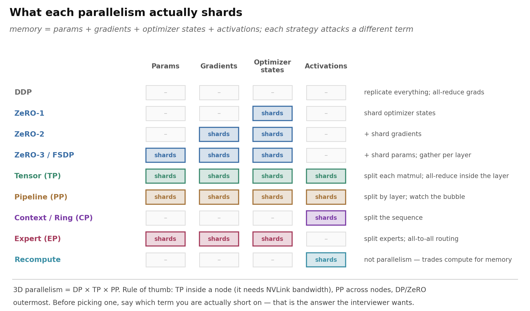 Figure 8. Every strategy attacks a different term. Naming the term before naming the strategy is the answer the interviewer is listening for.
- DDP replicates everything and all-reduces gradients. Simple, and it does nothing for memory.
- ZeRO [40] shards the optimizer state (stage 1), then gradients (stage 2), then parameters (stage 3), gathering each layer’s parameters just in time. FSDP [58] is PyTorch’s native implementation. Stage 3 trades communication volume for memory.
- Tensor parallelism [48] splits individual matmuls across devices. It needs an all-reduce inside every layer, so it wants NVLink-class bandwidth — keep it within a node.
- Pipeline parallelism [19] splits by layer. The cost is the bubble: with naive scheduling, devices idle while waiting for the stage before them. Micro-batching and 1F1B schedules shrink it; the bubble fraction is roughly \((p-1)/m\) for \(p\) stages and \(m\) micro-batches.
- Context / ring attention [31] splits the sequence, which is the only thing that helps when a single sequence’s activations do not fit.
- Expert parallelism distributes MoE experts, with all-to-all routing. The all-to-all is the bottleneck and the reason capacity factors exist.
- Activation recomputation [24] is not parallelism at all — it discards activations and recomputes them in the backward pass, trading roughly 30% more compute for a large memory saving.
3D parallelism is DP × TP × PP composed. The standard layout: TP innermost within a node, PP across nodes, DP outermost.
Numerics
Mixed precision [35] is the other half of making a large run fit, and it is asked because the failure modes are specific and memorable.
The scheme is: keep an fp32 master copy of the weights, run the forward and backward in reduced precision, and apply the optimizer update to the master copy. You do this because the update is typically many orders of magnitude smaller than the weight, so adding it in fp16 rounds it straight to zero — your model simply stops learning while the loss curve looks plausible.
Why bf16 beat fp16. They are the same width, but they split it differently: fp16 has 5 exponent bits and 10 mantissa bits, bf16 has 8 and 7. Eight exponent bits gives bf16 the same dynamic range as fp32, which means no overflow in the attention logits and no loss scaling machinery at all. You pay in mantissa precision, and it turns out training does not care much. With fp16 you need dynamic loss scaling — multiply the loss before the backward pass to lift small gradients into representable range, then unscale before the optimizer step, and back off the scale whenever you see an inf. That machinery is a recurring source of “the run silently stopped improving” bugs, which is why the field moved.
What must stay in fp32. Reductions. Softmax denominators, layer-norm and RMSNorm statistics, loss accumulation, and gradient all-reduce. This is why the RMSNorm implementation earlier casts back with .type_as(x) — the reduction happens in higher precision and only the result is narrowed.
FP8 is the current frontier: DeepSeek-V3 trained at scale with an FP8 mixed-precision framework [8], using per-tile and per-block scaling rather than one global scale, because FP8’s range is narrow enough that a single scale factor cannot cover a whole tensor. If asked about it, the honest answer is that the gains are real and the numerical engineering is genuinely hard.
MFU is the number that summarizes whether any of this is working: achieved FLOP/s divided by the hardware’s peak. Compute the numerator as roughly \(6 \times P \times D\) FLOPs for \(P\) parameters and \(D\) tokens (a forward-backward pass is about 6 FLOPs per parameter per token; add ~2 more if you are recomputing activations). Something in the 35–50% range is healthy for large-scale training. When it is low, the causes are almost always: communication not overlapped with compute, pipeline bubbles, a data loader that cannot keep up, or too-small per-device batches.
Debugging a loss spike
Here is E2 in full, because it is the most commonly reported “hard” mechanism question and it has a structure you can actually rehearse.
“You are pretraining a 100B model. At step 42,000 the loss spikes. What do you do?”
The wrong answer is to immediately propose lowering the learning rate. The right answer starts by classifying the spike, because the three shapes have different causes and different responses.
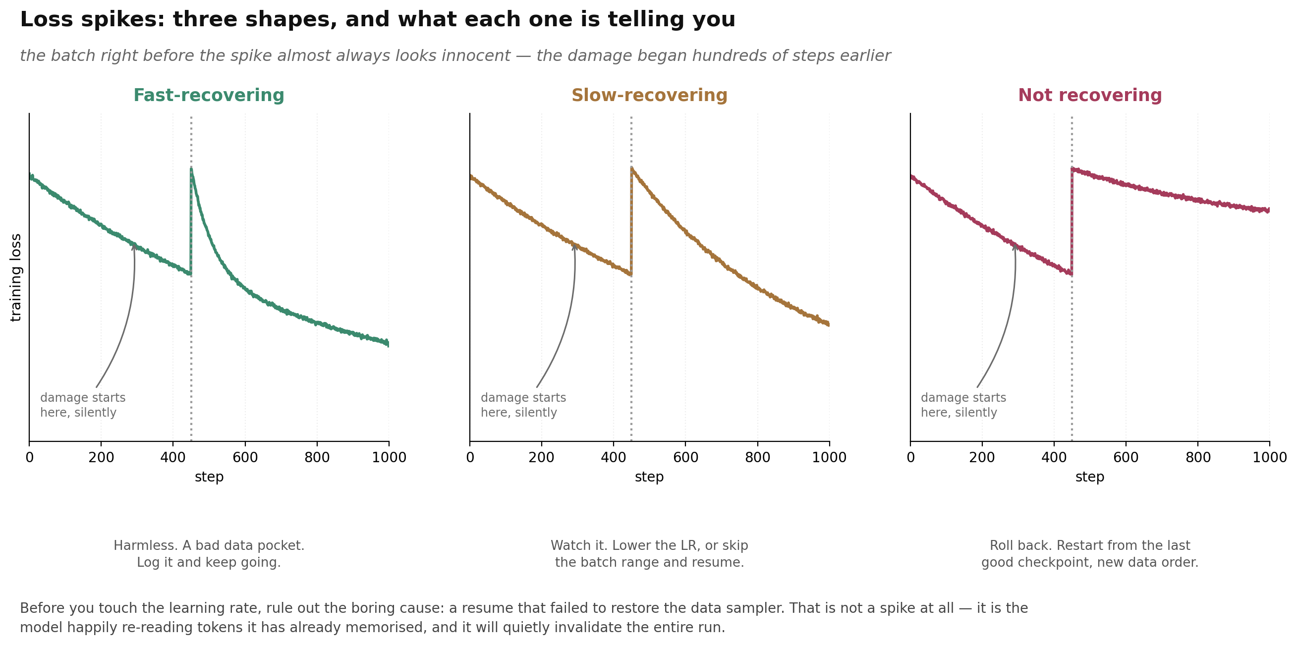 Figure 9. Bekman’s taxonomy [4]. The critical subtlety: the batch immediately before the visible spike almost always looks innocent, because the problem started developing hundreds of steps earlier.
Bekman’s open book on ML engineering [4] — written out of training BLOOM-176B and IDEFICS-80B, and the best public reference on this — gives three types: fast-recovering, slow-recovering, and not fully recovering. His diagnosis of the usual cause:
“The spikes usually happen because of a bad data pocket, either due to badly shuffled data or because it hasn’t been cleaned from some garbage scraped from the websites.” [4]
And the subtlety that makes this a good interview question:
“While one would suspect that the batch before the spike was the trigger, but if you were to study that batch’s contents you are likely to find nothing unusual - quite often the problem starts developing many steps before and then most of the sudden it happens.” [4]
A structured answer walks the ladder from cheapest to most expensive:
- Is it real, or is it logging? Check whether the spike appears in the gradient norm and in validation loss, or only in a smoothed training curve on one rank.
- Is it a resume artifact? This is the highest-value check and almost nobody mentions it. If the run restarted and the data sampler did not restore its position, the model is re-reading tokens it has already seen. Bekman’s warning is stark: you can discover after the fact that you trained “6x times the same 50B of tokens from the planned 300B tokens seen only once each” [4]. That is not a spike pathology, it is a silently invalidated run.
- Is it hardware? A single flaky GPU producing bad gradients will poison the all-reduce. Check per-rank loss, look for ECC errors, and run a collective-communication benchmark.
- Is it numerics? In fp16, overflow in the attention logits or the loss scaler collapsing. Check for inf/NaN in the gradients before clipping. This is a large part of why bf16 replaced fp16 — same dynamic range as fp32, so no loss scaling needed.
- Is it data? Now go look at the batches in the window before the spike, not the batch at it. Long runs of repeated tokens, a corrupted shard, or a language switch are typical.
- Only then, optimization. Is the LR too high for the current curvature? Has the second-moment estimate gone stale after a schedule change? Did a warmup restart get skipped?
And the responses, matched to the classification: for fast-recovering, log it and continue. For slow-recovering, consider lowering the LR or skipping the offending data range. For non-recovering, roll back to the last good checkpoint and resume with a different data order — and note that you should already have a policy on checkpoint frequency, because this is a question of how much compute you are willing to lose.
The meta-point worth making out loud: check the public training logbooks. Bekman maintains a collection of them precisely because your instability is probably already documented with a known mitigation [4]. Saying “I’d check whether this is a known failure mode before theorizing” is a better-engineer answer than any specific hypothesis.
Question bank
Why is the value function hard to train for LLMs? Rewards are sparse (one scalar for an entire response), the target distribution shifts as the policy improves so the critic always lags, and it is another full-size model in memory. All three arguments point at GRPO.
When is GRPO a bad choice? When rewards are dense or per-token, when you cannot afford \(G\) samples per prompt, and when reward variance within groups is low — which makes most groups contribute nothing. For preference-based rewards without a verifier, GRPO works but its advantage over PPO is much less obvious.
How do you choose the KL coefficient? Don’t pick it by taste — target a KL value. Monitor the actual KL divergence from the reference and adapt β to hold it near a target. If KL is near zero the model isn’t learning; if it’s climbing without bound you will get reward hacking and capability loss.
What is the difference between the KL in PPO and the KL in GRPO? Placement (reward versus loss), estimator (raw versus k3), and granularity. This is the single most reliable “did they actually implement this” question.
Why do we need a reference model at all? To bound drift from the SFT policy. Without it, optimizing a learned reward model will find its failure modes, and the policy will lose general capability while the reward number goes up.
Explain the full RLHF pipeline. Pretrain, SFT on demonstrations, collect preference comparisons on policy samples, train a Bradley-Terry reward model, then PPO against that reward with a KL penalty to the SFT policy [37]. Then say what has changed since: verifiable rewards where possible, GRPO instead of PPO in reasoning work, DPO where you have static preference data and want simplicity, and iterated rounds rather than one pass [28].
What is the bubble in pipeline parallelism and how do you shrink it? Idle time while a stage waits. Shrink with more micro-batches, an interleaved 1F1B schedule, or zero-bubble schedules that split the backward pass into input-gradient and weight-gradient halves.
Why bf16 over fp16? Same exponent range as fp32, so no loss scaling and far fewer overflow failures, at the cost of mantissa precision that turns out not to matter much for training. Keep fp32 master weights and do reductions in fp32.
Takeaway. Anyone can name the algorithms. The signal is in the placement of the KL term, the shape of the advantage, and whether your first move on a loss spike is to check the data sampler.
Bucket 5: ML systems design
Classical system design has largely been replaced in these loops. One candidate account puts it about as bluntly as it can be put: nobody asked them to design a URL shortener, nobody asked about a chat service; the question was inference-serving infrastructure for millions of requests across differently-sized models while keeping GPU utilization high — batching, KV-cache memory management, routing, and how latency compounds through a transformer pipeline.
Two things follow from that. First, the interviewer has built the real version. Reported experiences consistently mention being caught out within a couple of minutes for having prepared from generic material. Second, the prompts cluster tightly: batching GPU requests, inference systems, model downloaders, prompt playgrounds, evaluation harnesses.
Prefill and decode are two different machines
If you internalize one thing from this section, make it this. Almost every serving decision falls out of a single distinction, and stating it in the first two minutes reframes the whole conversation.
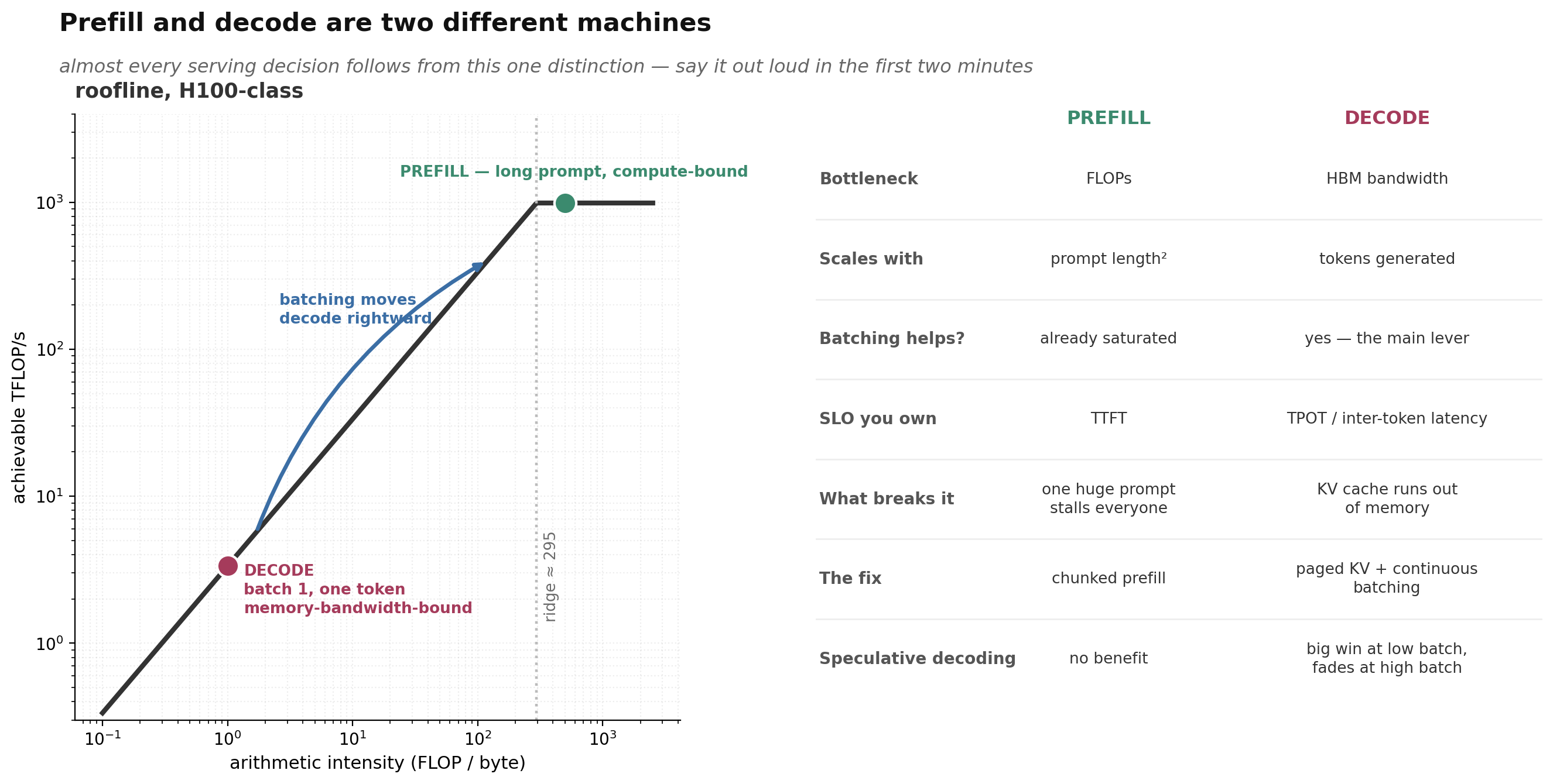 Figure 10. Prefill processes the whole prompt in parallel and saturates the GPU’s arithmetic units. Decode produces one token at a time and spends its life waiting on memory. They have different bottlenecks, different SLOs, and different fixes.
Prefill processes the prompt. Every token attends to every other token, so there is a large amount of parallel work per byte of weights read. Arithmetic intensity is high, you sit to the right of the roofline’s ridge point, and you are compute-bound. Cost grows with the square of prompt length.
Decode generates one token. You read the entire weight matrix — tens of gigabytes — to compute a single token’s worth of arithmetic. Arithmetic intensity is terrible, you are far to the left of the ridge, and you are memory-bandwidth-bound. The GPU’s FLOPs are almost entirely idle.
That single fact explains essentially the whole serving stack:
- Batching is the main decode lever, because it amortizes the weight read across many sequences, moving you rightward on the roofline. It does almost nothing for prefill, which is already saturated.
- Continuous batching exists because static batching wastes the tail: with a fixed batch, short sequences sit idle waiting for the longest one to finish. Continuous batching evicts finished sequences and admits new ones at each step.
- KV-cache paging [25] exists because the cache is the thing that limits how many sequences you can batch, and naive contiguous allocation fragments badly — you must reserve for the maximum possible length. Paging the cache into fixed-size blocks, exactly like virtual memory, removes the fragmentation and makes copy-on-write prefix sharing possible.
- Chunked prefill exists because one enormous prompt monopolizes the GPU and stalls everyone else’s decode steps, wrecking inter-token latency for every concurrent user.
- Prefix caching exists because the shared system prompt is recomputed for every request otherwise.
- Disaggregated prefill/decode exists because the two phases want different hardware ratios and interfere with each other on shared devices.
- Speculative decoding [29] exists because decode has idle FLOPs. A small draft model proposes several tokens, the large model verifies them in a single parallel forward pass, and you use the spare arithmetic to buy tokens. The critical caveat, and the follow-up they will ask: its benefit shrinks as batch size grows, because at high batch you are no longer bandwidth-starved and there are no spare FLOPs to exploit.
The two SLOs you own are TTFT (time to first token, governed by prefill and queueing) and TPOT (time per output token, governed by decode). They trade against each other, and throughput trades against both. Naming which one the product cares about is the first question you should ask.
Worked design: serve a family of models
Here is the reported Anthropic-style prompt, worked the way I would work it.
“Design an inference service that serves several model sizes to millions of requests per day while keeping GPU utilization high.”
Step 1: clarify, then do the arithmetic out loud. This is the step candidates skip, and it is the one that signals experience. Ask: how many models and what sizes? What is the request rate and its peak-to- average ratio? What is the prompt-length and output-length distribution? Interactive or batch? What is the latency SLO, and is it on TTFT or end-to-end? Is there a shared system prompt?
Then commit to numbers and compute. Say 100M requests/day — about 1,150 requests/second average, call it 3,500/second at peak. Say a 70B model in bf16: 140 GB of weights, so it does not fit on one 80 GB device and needs tensor parallelism across at least two, realistically four. With GQA at 8 KV heads, the cache is 320 KB per token, so a 10k-token context costs about 3.2 GB per sequence. On 4×H100 you have 320 GB total, minus 140 for weights, leaving roughly 160 GB of usable KV space after overhead — about 50 concurrent sequences at that context length. If a request occupies a slot for 5 seconds, one 4-GPU replica serves roughly 10 requests/second, so peak demand needs on the order of 350 replicas, or 1,400 GPUs. Now you have grounds for an architecture, and you have shown you can size a system.
Step 2: the request path. Gateway (auth, rate limiting, quota) → router → per-model replica pools → scheduler → engine. The router’s job is model selection and load-aware placement; the scheduler’s job is admission and batching.
Step 3: the scheduler, which is where the real content is. Continuous batching with paged KV. A running batch that admits new requests whenever cache blocks free up. Chunked prefill so long prompts are broken into pieces and interleaved with decode steps rather than blocking them. Priority classes if you have interactive and batch traffic sharing hardware. And an explicit preemption policy for when the cache fills: either recompute the evicted sequence’s prefill later, or swap its blocks to host memory. Knowing that this decision exists is a strong signal.
Step 4: multi-model. The naive approach dedicates GPUs per model, which wastes capacity when traffic is skewed. Options to raise and evaluate: separate pools with autoscaling (simple, slow to adapt); multiplexing several models on a device (only viable for small models; the KV cache makes it hard); LoRA-style multi-tenancy where many adapters share one base model’s weights (excellent when the variants are fine-tunes); and cold-start mitigation, because loading 140 GB of weights takes minutes — you need warm pools, and a model-downloader/cache service, which is itself one of the reported prompts.
Step 5: what breaks. A single very long request holding cache blocks for minutes. A traffic spike that fills the cache and triggers a preemption storm. A bad node degrading the whole tensor-parallel group — TP is synchronous, so the slowest device sets the pace. Head-of-line blocking in the queue. And the cost question: what is your dollars-per-million-tokens, and which knob moves it most? (Usually batch size, then quantization, then speculative decoding at low load.)
Step 6: what you would measure. TTFT and TPOT at p50/p95/p99, not the mean. Tokens/second/GPU. KV cache utilization and preemption rate. Batch size distribution. Queue depth. Goodput — requests served within SLO, which is the metric that actually matters and the one candidates rarely name.
Question bank
Design a training cluster for a 100B model. Work the memory equation first: ~16 bytes/parameter with AdamW and fp32 master weights means 1.6 TB before activations, so you need model sharding, not just data parallelism. Then the layout: TP=8 within a node, PP across nodes, ZeRO/FSDP for the rest. Then the parts people forget — checkpointing frequency versus restart cost, the data pipeline’s throughput (it must keep thousands of GPUs fed), failure detection and automatic restart, and monitoring MFU as the health metric.
Design an evaluation harness for a coding agent. Sandboxed execution is the whole problem: containers with no network, resource limits, timeouts. Then determinism — pinned dependencies, fixed seeds, and a policy for flaky tests. Then the eval-latency problem: if a task takes an hour, you cannot iterate, so you need parallelism across tasks and a fast smoke subset. Then contamination: benchmarks built from public repositories may already be in the training data, so you need held-out tasks created after the cutoff.
Design a RAG system, then break it. The design is standard; the interesting half is the failure taxonomy. Retrieval misses (fix: hybrid BM25 plus dense, query rewriting), retrieval succeeds but the generator ignores the context (fix: instruction tuning, citation requirements), chunk boundaries splitting the answer (fix: overlapping chunks, or parent-document retrieval), and stale indexes. Then evaluation: retrieval quality and generation quality must be measured separately, or you cannot tell which half is broken.
How would you cut inference cost by 50%? In order of effort-to-payoff: raise batch size until the latency SLO binds; enable prefix caching if there is a shared prompt; quantize weights to INT8 or FP8; route easy queries to a smaller model; add speculative decoding if load is low and interactive; and only then consider distillation. Say which one you would try first and why.
Takeaway. Do the arithmetic before the architecture, and say the prefill/decode distinction out loud early. The person across the table has operated this system and can tell within two minutes whether you have.
Bucket 6: Research taste, deep dives, and values
This is the bucket that decides the loop, and the one that cannot be crammed. Meng’s assessment is worth sitting with:
“Coding interviews weed out weak candidates, but exactly no one gets hired because they did well on coding. Design interviews test your first-principles thinking, but you might never have had success in this domain yet. Project deep dives, by contrast, show exactly why you’re the right person for this team.” [34]
The research presentation
For research-track roles you may be asked for a job talk on your own work: roughly ten slides, defended like a thesis. Meng describes it as “a job talk style presentation on your past work… you ‘defend’ your body of work like a PhD candidate would” [34].
A structure that works:
- The problem, and why it was not already solved. One slide. If the audience does not care by the end of it, nothing else lands.
- Your specific contribution, stated as a claim you can defend rather than a list of activities.
- Method, with the one design decision that mattered given a full slide of its own.
- Results, including the baseline you almost lost to.
- What did not work, and what you learned. This slide is the one that distinguishes researchers from people who report results.
- What you would do next, and how you would know if you were right.
The most common failure is presenting a chronology instead of an argument. The second most common is being unable to answer “what is the weakest part of this?” — have a real answer, because the strongest signal you can send is that you have already been your own harshest reviewer.
The paper round
Some labs send a paper in advance; others hand you one live. Either way the bar is not “what does it say.” It is what would you do next.
A reusable frame, which also works when you have not read the paper:
- Claim. What exactly is being asserted? Separate the empirical claim from the interpretation the authors put on it.
- Evidence. What experiment supports it? What would falsify it? Is the baseline fair — same compute, same data, same tuning effort?
- Mechanism. Why would this work? If the authors offer an explanation, does it predict anything else they did not test?
- Scope. What breaks at 10× scale, or on a different modality, or with a stronger base model?
- Next. The one experiment you would run, and what each outcome would tell you.
Jaiswal’s system for staying current is the most practical thing I found on this, and worth adopting whole. She maintained a section she deliberately called “I know of these papers” — the word “know” chosen because it “captures multiple levels of familiarity: deeply reading papers, skimming them, finding them through social media, learning about them from others’ presentations or discussions, and implementing them firsthand” [21]. Paired with an honesty rule that I think is genuinely good interview advice:
“When interviewers ask open-ended questions, I make a point to cite my sources, saying things like ‘I learned this from a blog post’ or ‘I’ve seen this discussed widely on Twitter.’ I maintain a broad collection of references and always stay transparent about my depth of understanding for each paper.” [21]
Calibrated confidence reads as strength, not weakness. “I’ve only skimmed this one, but my understanding is X — is that right?” is a much better answer than confident vagueness, and it invites the interviewer into a conversation rather than an examination.
The project deep dive
Every loop has one, and it is the highest-leverage round for most people because it is the only one where your actual experience is the material.
The pattern reported repeatedly is relentless drilling: the interviewer keeps asking why until they hit either bedrock or your limit. What did you specifically do, as opposed to your team? Why that design and not the obvious alternative? What was the trade-off? How did you measure it? What went wrong? Staying at a high level is read as not having gone deep.
Preparation that works: write the project out longhand, everything that happened, then organize it into chapters — design, development, launch, learnings, next steps — and separate the technical complexity from the collaboration complexity, because interviewers probe both. Then find the two or three decisions where you chose one path over another and be able to defend both sides.
The hardest question in this round is usually: “What would you do differently?” An answer that is actually a humblebrag fails. An answer that identifies a real mistake, explains what you misjudged and what you now believe instead, passes.
The values round
Nobody prepares for this as a technical round. It is repeatedly reported as failing more technically strong candidates than any coding round.
Three reasons it fails people. It is not a culture-fit chat, so STAR stories about team conflicts do not land. It probes reasoning rather than conclusions, so the follow-up to whatever you say is “why?” and then “what would change your mind?” And it is detectable when memorized — questions like “a belief you changed,” “a genuine critique of this company,” or “what failure mode of LLMs worries you most, and what changes when you give an agent tool use” cannot be answered from a script.
What actually prepares you:
Read the primary sources, and disagree with something specific. Constitutional AI [3] and InstructGPT [37] if you are talking to Anthropic or OpenAI respectively; the model cards and system cards; the published safety frameworks. Anthropic’s own candidate guidance explicitly suggests using Claude to build a study guide covering “key topics I should review, including AI safety concepts, [the company’s] research focus” [2] — so this is expected of you, not optional. But reading is the floor. Having one specific, well-reasoned disagreement is the signal.
Form a position on something concrete rather than something general. “I care about AI safety” is noise. “I think the strongest current argument against RLHF as a safety mechanism is that it trains the model to produce outputs humans approve of, which is a different target from outputs that are correct — and as tasks exceed human ability to evaluate, that gap widens rather than closes” is a position. It can be argued with, which is the point.
Be able to hold uncertainty. The round is testing whether you can reason under genuine uncertainty without collapsing into either false confidence or refusal to commit. The move is to state your view, state your confidence, and state what evidence would move you.
Have real stories, honestly told. A time your values were tested. A time you were wrong about something that mattered. A decision you would make differently. These need to be true, because the follow-ups go three levels deep and invented stories run out of detail.
Takeaway. This bucket has a lead time measured in months and cannot be compressed. It is also the one where the preparation is indistinguishable from just being a thoughtful person about your field — which is why starting it first costs you nothing.
Bucket 7: Math
I had not seen this written down anywhere until Liu listed it as its own category:
“Some companies have a math interview, ranging from fun logic puzzles to serious mathematical derivations with pen and paper. I would recommend brushing up on probability, linear algebra, and calculus.” [30]
She wrote an entire separate set of notes for it, “all for a single fateful interview” [30] — which tells you both that it is real and that it is rare enough to be a nasty surprise. Sapora’s topic list independently carries a full linear-algebra block: positive semi-definiteness, Jacobian, Hessian, eigenvectors and eigenvalues, null space and image space, orthogonality, linear independence, singular matrices, rank and span, determinant [42]. Lambert saw the same thing in 2022, describing companies running “‘ML Background’ interviews that are mostly math tricks and basic ML tradeoffs” and admitting “Preparing for this is hard, but studying some coursework would help. I didn’t” [26].
The scope is narrower than a qualifying exam. What actually recurs:
Probability. Expectation and variance, and specifically being fluent with linearity of expectation as a proof device. Conditional probability and Bayes. Common distributions and when each arises. The concentration inequalities by name (Markov, Chebyshev, Hoeffding) and what each buys you. Markov chains and stationary distributions. And the classic puzzle family — expected number of coin flips to see a pattern, the ballot problem, birthday-collision arguments — which is what “fun logic puzzles” usually means in practice.
Linear algebra with an ML accent. Eigendecomposition and SVD, and crucially what they mean rather than how to compute them: SVD gives you the best low-rank approximation, which is why LoRA is plausible at all, and why PCA works. Positive semi-definiteness and why covariance matrices and Hessians at minima are PSD. Rank, null space, and why a rank-\(r\) update has \(r(m+n)\) parameters. Matrix calculus: the Jacobian, the chain rule in matrix form, and the handful of derivative identities you need to derive a backward pass without looking anything up.
Calculus and optimization. Gradients and Hessians, convexity and why it matters (and why nobody has it), Taylor expansion as the justification for gradient descent, Lagrange multipliers, and Jensen’s inequality — which shows up constantly because it is the engine behind the ELBO.
Information theory. Entropy, cross entropy, KL divergence. Be ready for the question that Sapora says she got wrong and cried about afterwards, because it is the canonical one: why is forward KL mean-covering and reverse KL mode-seeking? The answer is in where the infinite penalty sits. Forward KL, \(D_{KL}(p \| q)\), weights by \(p\), so wherever \(p\) has mass and \(q\) does not you pay enormously — the fitted \(q\) must therefore cover all of \(p\)’s support, smearing across modes. Reverse KL, \(D_{KL}(q \| p)\), weights by \(q\), so \(q\) is punished for putting mass where \(p\) has none but pays nothing for ignoring a mode entirely — it collapses onto one. Maximum likelihood is forward KL; variational inference and the RLHF KL penalty are reverse. That she got this wrong “after dealing with forward vs reverse KL in two separate papers” [42] is the whole argument for rehearsing things you already know.
Takeaway. Small surface, high variance. A weekend of probability and linear algebra revision is cheap insurance against a round you may not be told about in advance.
Gate 3: timing, work trials, and negotiation
Everything up to here is the part people prepare for. This is the part that, by the accounts of everyone who has been through it recently, determines a surprising fraction of the outcome — and almost nobody rehearses it.
Sequencing your companies
The standard advice is to use a few companies as practice and time the rest so offers land together. Liu says that is roughly right in spirit and then adds three corrections that matter more than the rule [30]:
Your stamina is finite. “Practice interviews are helpful, but also recognize that your stamina is finite — be careful not to burn out by the time you get to places you really care about!” Sapora runs the same play with a refinement: start with “Smaller startups, companies in locations you’re not keen on, roles that are interesting but not your top choice” — you calibrate your confidence and learn what compensation looks like before it counts [42].
External factors can outweigh your preparation. “There are external factors to timing that are worth taking into account, such as whether the company has headcount and which teams are actively hiring, and this can matter more than your preparation” [30]. Yong independently lands on the same point and says to ask recruiters about headcount directly [55]. Lambert confirms it from the inside: companies hit “total headcount locks mid cycle,” and you should talk to others searching in your area so you know it is not you [26].
Deadlines have more give than they look. Liu: “Deadlines come with a lot of flexibility… Recruiters recognize you have other processes to finish, and there are various tricks to delay the offer and decision” — with the caveat to investigate exploding offers specifically [30]. Sapora saw deadlines ranging from one week to “take a reasonable amount of time” and found companies inflexible about extending, though friends of hers did get extensions [42]. So: treat flexibility as likely but not guaranteed, and find out early.
Two more operational rules. Tell every company about your other processes — Sapora: “I know it feels uncomfortable for some people but it’s completely normal and expected. It keeps timelines clear, encourages processes to chug along nicely, and often prompts companies to move faster if they’re interested” [42]. And one interview per day if you can manage it: “interviews are exhausting and you are naturally going to underperform in your third interview of the day” [42].
Yong’s warning about compression is the counterweight: “Don’t be surprised if you have to have three back-to-back interviews within a single day, and you only have less than a day to prepare for them” [55]. Pushing the start of a process back a month or two is normal; once it starts, the gaps are short.
And one thing you are allowed to do that candidates forget, from Lambert: “You can say no to companies. If they’re doing something ridiculous like not communicating the schedule or saying they only have 1 timeslot for an interview, ask them to make space for you” [26].
Work trials
I had dismissed these as an invention of the content farms, because only content farms mentioned them. They are real, and Yong describes them as the biggest surprise of his search [55]:
“Work trials are completely different from onsite — you are not flown to the company to do multiple interview rounds onsite; instead, you are working with the team to solve a task. Sometimes, the task can be open-ended. These work trials are paid usually, but what surprises me is that some of these in-person work trials can last up to a week.”
The practical consequence is the part to internalize, because it wrecks scheduling:
“doing work trials make it really hard to prepare for other companies’ interviews as I would have to put in my everything on the current task assignment and have no bandwidth for interview prep with other companies.” [55]
If a trial is in your pipeline, treat it as a blackout window and sequence everything else around it. And note that a trial is an evaluation running in both directions — a week inside the team tells you more about whether you want the job than any number of team-match calls.
Negotiation
This is the highest-value-per-hour work in the entire process, and the least prepared-for. Liu’s passage on it is the single most useful thing in any of these posts:
“The truth is that negotiating is hard. Nothing in our PhD prepared us for this, and unlike interviews, this part cannot be conquered by studying. Compared to recruiters, you are outmatched in both knowledge of the market and the skill of negotiation, and everyone you talk to wants something different from you. You may be thinking, ‘I would be happy with my offer and make a decision independently of compensation!’, and indeed it’s great to know your own values! But you’d be doing yourself a disservice if you didn’t negotiate. Initial offers leave room for negotiation by design; recruiters often explicitly invited me to play the game by saying things like, ‘I don’t expect you to take our first offer.’ Putting in energy here for a few weeks can, literally, be equivalent to years of work at the initial offer.” [30]
Her method is the transferable part, and it is just interview preparation pointed at a different target:
“Before every recruiter call, I wrote down what I was willing and not willing to share, along with quotes I could recite verbatim. In the post-offer stage, I would anticipate questions they might ask and points they might make, and carefully construct responses that I could deliver comfortably while still advocating for myself.” [30]
Note also that the post-offer stage is itself substantial work — she logged 16 post-offer chats on top of everything else, and describes “managing an overwhelming amount of communication” [30].
Sapora’s experience adds three empirical corrections to the usual advice [42]:
The blind-auction strategy did not survive contact. The standard advice is to never reveal competing offers. “That didn’t work for me: several companies explicitly asked for proof of other offers before increasing theirs, and one even questioned my screenshots.”
Companies have data on you that you don’t have on them. “If you tell Anthropic you’re seriously considering an offer from Peppers Burgers, they have data on how often candidates with both offers actually chose the latter. If the answer is ‘almost never,’ your bluff doesn’t work.” The corollary is that a competing offer only carries weight if it is from a genuine peer.
You are being read continuously. “Recruiters are surprisingly good at reading you… even small signals matter: how often you mention a company, how you talk about them, all of it gets noted. If a recruiter knows their company is already your preferred choice, negotiating is going to be harder.”
The one thing both of them say without qualification: companies move their numbers significantly if they want you, and it is always worth asking.
Two more things that belong here. Lean on friends — Liu: “It is really crucial at this stage to lean on your friends for the know-how of interacting with recruiters and for more data points to help calibrate your asks” [30]. And on choosing between offers, Sapora’s honest account of asking everyone at both companies: “every single person at DeepMind told me they’d choose DeepMind, and every single person at Isomorphic told me they’d choose Isomorphic. Extremely helpful.” What actually resolved it was talking to people who knew her [42].
Takeaway. Budget two weeks for this and rehearse it like a technical round. It is the only part of the process with a direct, immediate, and permanent financial return.
The part nobody prepares for
Both Liu and Sapora devote real space to the psychological cost, and both are unusually direct about it. I am including it because it is the most consistently reported and least written-about part of the process, and because reading it in advance is itself a form of preparation.
Liu:
“In this blog post I focused on the concrete parts of the job search, but in reality a huge part of my personal experience was managing all the emotions that come with being on the market. There is a lot of social perception to navigate: it is not a good feeling to compare yourself to your peers, everyone has opinions on where you should or shouldn’t go, and people become unusually invested in how your life is going… Frankly, I was stressed, miserable, and not functioning in other parts of my life for several months. Hopefully you find more joy, but if not, just know that you are not alone.” [30]
Sapora is more granular about the mechanics of it. She could not sleep the night before interviews, which becomes structural “when you have 10 interviews in a week.” She could not eat, and got nauseous at the sight of food. Her workarounds were exercise (“Running before interviews helped me a lot, it burned off nervous energy and reset my head”), a consistent evening routine, a fixed pre-interview ritual, and a rule to have dinner with friends any evening without a morning interview [42]. Then the harder part:
“At a certain point my anxiety was holding me back more than my preparation was. My mind would occasionally go blank mid-interview… In hindsight, that kind of reflection is more useful *before you start (knowing your triggers, your relationship with failure, what your sense of worth is actually tied to) so you’re not discovering it under fire like I did.”* [42]
Three things worth extracting as actual advice.
Sleep beats last-minute cramming, and it is not close. Liu did her first technical interview on two hours of sleep after cramming LLM inference internals: “none of the last-minute knowledge came up, and I ended up spending 10 minutes on an off-by-one error because my gears were barely turning” [30]. The expected value of one more hour of revision at midnight is negative.
The process is stochastic, and its verdict is not information about you. Sapora, having messed up a forward-versus-reverse-KL question she had literally published on: “your worth as a human being is not going to be decided by these interviews… You will mess up, even on things you know, and that’s okay” [42].
Do the introspection before, not during. This is her clearest piece of advice and the one that costs nothing to act on. Knowing in advance how you respond to failure is worth more than another twenty LeetCode problems.
I would add one observation from the sourcing itself. Liu, Sapora and Yong all published these accounts after succeeding — offers from OpenAI, DeepMind, and a lab of his choosing respectively. If the people who did unambiguously well describe the process as miserable, then finding it miserable is not evidence that it is going badly.
Takeaway. Plan for a months-long process that will be unpleasant even if it goes well, and set up the sleep, exercise, and social scaffolding before you need it rather than after.
Sequencing your preparation
The buckets have very different lead times, and lead time — not importance — should drive the order.
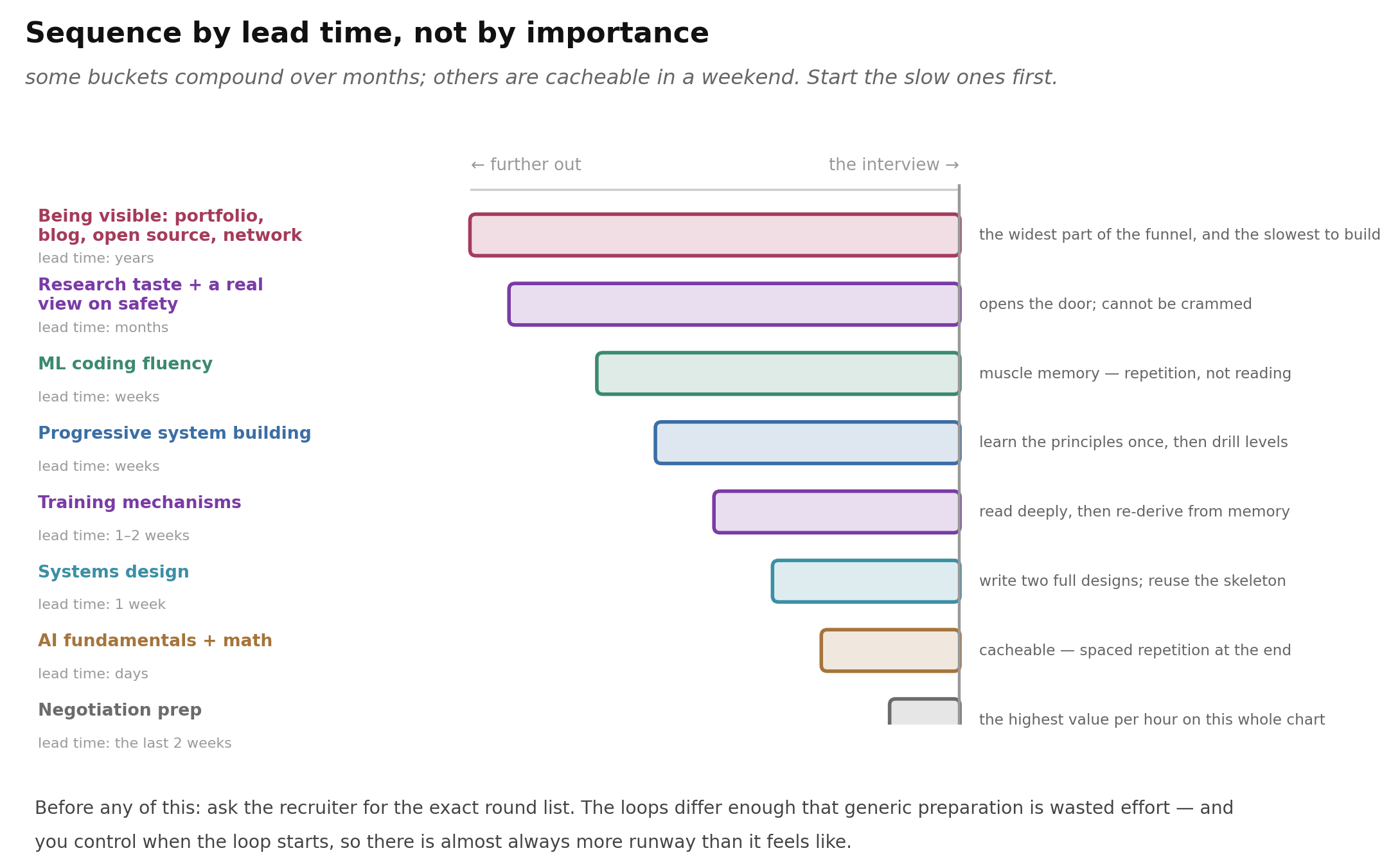 Figure 11. Visibility compounds over years and cannot be rushed. Negotiation is two weeks of work with the highest return per hour on the chart. Fundamentals are cacheable and belong at the end. Most people run this exactly backwards.
The rules I would extract from all four accounts:
Get the round list first. Everything downstream depends on it, and preparing generically means over-investing in rounds you will not have.
Make ML coding muscle memory, starting early. This is the most-repeated technical advice across every source. Liu’s specific recommendation is the most actionable: watch Stanford’s CS336, Language Modeling from Scratch [50], and treat Assignment 1 as the highest-ROI single artifact — “implementing / debugging a transformer comes up so often in interviews that it will pay off massively to turn it into muscle memory and really isn’t worth losing points on” [30]. Sapora’s six-item baseline [42] is the checklist for when you are done: transformer end-to-end, causal/cross/self attention, flash attention, the attention backward pass, MLP forward and backward, and a training loop.
Practice with AI completely off. Liu, emphatically: “Make sure you are practicing coding with AI assistance completely off to mimic interview settings (you will underestimate your reliance otherwise)!” [30] This matches Anthropic’s stated policy for live rounds [2] and is, in 2026, probably the single most-violated piece of preparation advice.
Prepare per-interview, not generically. Sapora: “I did little generic prep. Almost everything was targeted at the next specific interview or company. This kept me focused and meant the material I was asked about was fresh on my mind” [42]. Liu describes the same rhythm: “each interview is a slightly different math or CS class, you never went to lectures, and now you have ~3 days to cram for the midterm” [30]. Both then note that you cover most of the material anyway by the end.
Use LLM mock interviews. Sapora paste the role, company and round description into Claude and had it interview her before each round: “There was surprisingly frequent overlap between those practice questions and what interviewers actually asked” [42]. Note the distinction from the previous rule — LLMs for simulating the interview is encouraged; LLMs inside your coding practice defeats the point.
Keep an honest question log. Jaiswal’s four grades — “Aced it,” “Took time,” “Didn’t get it,” “Just saw it somewhere” [21] — force you to separate recognition from recall, which is exactly the distinction a 25-minute round tests. Liu records notes after each interview for the same reason [30].
Keep a spreadsheet. Sapora’s top regret: “I was convinced I could track everything in my head. Technically yes, but a simple spreadsheet (companies to apply to, where you are in each process, deadlines, contacts) would have stopped me from forgetting to apply to places I was actually interested in” [42].
Budget at least a month, and expect it to feel like a full-time job. Sapora: “Allocate at least a month of regular study time” [42]. Liu: “For me and for most people I talked to, the job search is a full-time job” [30].
One genuinely cheering note to end the planning section on, from Liu, because it reframes the whole exercise as something other than a tax:
“Studying carried enormous side benefits for me. Having a wider breadth of knowledge directly improved my confidence as a researcher… Amazingly, I also found that studying made me enormously more effective at my ongoing project. I was able to have technical ideas that I never would have been able to access before and do more technical work, which was thrilling.” [30]
Meng arrives at the same principle from a different direction: “every minute I spend on interview prep should make me a better engineer… Memorizing answers doesn’t do that for me” [34]. If your preparation plan does not pass that test, it is the wrong plan.
What I would still get wrong
Stated plainly, because a post like this should not pretend to more certainty than it has.
The record is thin, recent, and self-referential. There are perhaps five genuinely detailed first-hand accounts in existence, three of them published within a month of each other in mid-2026, and they cite one another. Liu’s timeline figure is modeled on Lambert’s; Yong’s post is explicitly written as a complement to Liu’s and Sapora’s. That is a healthy citation graph for a literature, but it is still a very small sample, drawn almost entirely from PhD candidates at strong programs who succeeded. Everyone whose search went badly is missing from the sample, and that is the most important limitation on everything above.
I missed these sources on my first pass, which should lower your confidence in my search, not raise it. I found the second tier and built a whole draft on it before being pointed at the primary layer. There may well be a third layer I still have not found.
The rounds genuinely are not standardized. Yong’s central point cuts against the neatness of any bucket taxonomy, including mine. Seven buckets is a useful organizing device, not a specification. Budget for the wildcard.
Nobody knows how AI-assisted rounds are scored. Meta’s version is documented; the rubric is not, and different interviewers within one company are almost certainly grading it differently right now. Meanwhile Anthropic’s live rounds are AI-free [2]. The two policies imply opposite preparation, and the industry has not settled.
Fit may dominate all of it. Meng’s single failed onsite was her best performance — wrong domain fit for the role [34]. Yong found that his award-winning papers had no bearing at all after he pivoted fields [55]. If the binding constraint is “Why you? Why not anyone else?”, then a large fraction of preparation effort is aimed at something other than the deciding factor. Meng’s conclusion — “Find a domain you love from the bottom of your heart and apply to roles in that domain” [34] — is either the deepest advice here or a rationalization of survivorship, and I cannot tell which.
This will age fast. GRPO post-dated Jaiswal’s loop entirely [21]. Work trials and AI-assisted rounds barely existed two years ago. Whatever the equivalent is in eighteen months, none of these sources can tell you.
References
- Ainslie, J., Lee-Thorp, J., de Jong, M., et al. (2023). GQA: Training Generalized Multi-Query Transformer Models from Multi-Head Checkpoints. arXiv:2305.13245
- Anthropic. Guidance on Candidates’ AI Usage. anthropic.com/candidate-ai-guidance
- Bai, Y., Kadavath, S., Kundu, S., et al. (2022). Constitutional AI: Harmlessness from AI Feedback. arXiv:2212.08073
- Bekman, S. (2023–2026). Machine Learning Engineering Open Book. github.com/stas00/ml-engineering
- Dao, T., Fu, D. Y., Ermon, S., Rudra, A., & Ré, C. (2022). FlashAttention: Fast and Memory-Efficient Exact Attention with IO-Awareness. arXiv:2205.14135
- Deep-ML. Practice Machine Learning. deep-ml.com
- DeepSeek-AI. (2024). DeepSeek-V2: A Strong, Economical, and Efficient Mixture-of-Experts Language Model. arXiv:2405.04434
- DeepSeek-AI. (2024). DeepSeek-V3 Technical Report. arXiv:2412.19437
- DeepSeek-AI. (2025). DeepSeek-R1: Incentivizing Reasoning Capability in LLMs via Reinforcement Learning. arXiv:2501.12948
- Fedus, W., Zoph, B., & Shazeer, N. (2021). Switch Transformers: Scaling to Trillion Parameter Models with Simple and Efficient Sparsity. arXiv:2101.03961
- Gordić, A. (2021). How I Got a Job at DeepMind as a Research Engineer (without a Machine Learning Degree!). gordicaleksa.medium.com
- Grattafiori, A., et al. (2024). The Llama 3 Herd of Models. arXiv:2407.21783
- Grigorev, A. (2026). AI Engineering Field Guide. github.com/alexeygrigorev/ai-engineering-field-guide
- Gupta, G. (2025). Notes on large-scale ML design and optimization for efficient training and inference. Shared via X and LinkedIn; see linkedin.com/in/gauri19
- He, K., Zhang, X., Ren, S., & Sun, J. (2015). Deep Residual Learning for Image Recognition. arXiv:1512.03385
- Hoffmann, J., Borgeaud, S., Mensch, A., et al. (2022). Training Compute-Optimal Large Language Models. arXiv:2203.15556
- Holtzman, A., Buys, J., Du, L., Forbes, M., & Choi, Y. (2019). The Curious Case of Neural Text Degeneration. arXiv:1904.09751
- Hu, E. J., Shen, Y., Wallis, P., et al. (2021). LoRA: Low-Rank Adaptation of Large Language Models. arXiv:2106.09685
- Huang, Y., Cheng, Y., Bapna, A., et al. (2018). GPipe: Efficient Training of Giant Neural Networks using Pipeline Parallelism. arXiv:1811.06965
- Huyen, C. (2021). Introduction to Machine Learning Interviews Book. huyenchip.com/ml-interviews-book
- Jaiswal, M. (2024). LLM (ML) Job Interviews — Resources. mimansajaiswal.github.io
- Kaplan, J., McCandlish, S., Henighan, T., et al. (2020). Scaling Laws for Neural Language Models. arXiv:2001.08361
- Karpathy, A. nanoGPT, micrograd, and Neural Networks: Zero to Hero. github.com/karpathy
- Korthikanti, V., Casper, J., Lym, S., et al. (2022). Reducing Activation Recomputation in Large Transformer Models. arXiv:2205.05198
- Kwon, W., Li, Z., Zhuang, S., et al. (2023). Efficient Memory Management for Large Language Model Serving with PagedAttention. arXiv:2309.06180
- Lambert, N. (2022). Job Hunt as a PhD in AI / ML / RL: How it Actually Happens. natolambert.com
- Lambert, N. (2026). Thoughts on the job market in the age of LLMs. Interconnects. interconnects.ai
- Lambert, N., Morrison, J., Pyatkin, V., et al. (2024). Tülu 3: Pushing Frontiers in Open Language Model Post-Training. arXiv:2411.15124
- Leviathan, Y., Kalman, M., & Matias, Y. (2022). Fast Inference from Transformers via Speculative Decoding. arXiv:2211.17192
- Liu, A. (2026). Notes on the Industry Job Search. alisawuffles.github.io
- Liu, H., Zaharia, M., & Abbeel, P. (2023). Ring Attention with Blockwise Transformers for Near-Infinite Context. arXiv:2310.01889
- Liu, J., Su, J., Yao, X., et al. (2025). Muon is Scalable for LLM Training. arXiv:2502.16982
- Loshchilov, I., & Hutter, F. (2017). Decoupled Weight Decay Regularization. arXiv:1711.05101
- Meng, Y. (2026). MLE Interview 2.0: Research Engineering and Scary Rounds. yuan-meng.com
- Micikevicius, P., Narang, S., Alben, J., et al. (2017). Mixed Precision Training. arXiv:1710.03740
- Milakov, M., & Gimelshein, N. (2018). Online normalizer calculation for softmax. arXiv:1805.02867
- Ouyang, L., Wu, J., Jiang, X., et al. (2022). Training language models to follow instructions with human feedback. arXiv:2203.02155
- Prince, S. J. D. (2023). Understanding Deep Learning. MIT Press. udlbook.github.io/udlbook
- Rafailov, R., Sharma, A., Mitchell, E., et al. (2023). Direct Preference Optimization: Your Language Model is Secretly a Reward Model. arXiv:2305.18290
- Rajbhandari, S., Rasley, J., Ruwase, O., & He, Y. (2019). ZeRO: Memory Optimizations Toward Training Trillion Parameter Models. arXiv:1910.02054
- Raschka, S. (2024). Build a Large Language Model (From Scratch). Manning. github.com/rasbt/LLMs-from-scratch
- Sapora, S. (2026). ML Job Interviews: The Ultimate Guide. silviasapora.github.io
- Schulman, J., Moritz, P., Levine, S., Jordan, M., & Abbeel, P. (2015). High-Dimensional Continuous Control Using Generalized Advantage Estimation. arXiv:1506.02438
- Schulman, J., Wolski, F., Dhariwal, P., Radford, A., & Klimov, O. (2017). Proximal Policy Optimization Algorithms. arXiv:1707.06347
- Sennrich, R., Haddow, B., & Birch, A. (2015). Neural Machine Translation of Rare Words with Subword Units. arXiv:1508.07909
- Shao, Z., Wang, P., Zhu, Q., et al. (2024). DeepSeekMath: Pushing the Limits of Mathematical Reasoning in Open Language Models. arXiv:2402.03300
- Shazeer, N. (2019). Fast Transformer Decoding: One Write-Head is All You Need. arXiv:1911.02150
- Shoeybi, M., Patwary, M., Puri, R., et al. (2019). Megatron-LM: Training Multi-Billion Parameter Language Models Using Model Parallelism. arXiv:1909.08053
- Snell, C., Lee, J., Xu, K., & Kumar, A. (2024). Scaling LLM Test-Time Compute Optimally can be More Effective than Scaling Model Parameters. arXiv:2408.03314
- Stanford University. CS336: Language Modeling from Scratch. cs336.stanford.edu
- Su, J., Lu, Y., Pan, S., et al. (2021). RoFormer: Enhanced Transformer with Rotary Position Embedding. arXiv:2104.09864
- Vaswani, A., Shazeer, N., Parmar, N., et al. (2017). Attention Is All You Need. arXiv:1706.03762
- Xiong, R., Yang, Y., He, D., et al. (2020). On Layer Normalization in the Transformer Architecture. arXiv:2002.04745
- Yang, G., Hu, E. J., Babuschkin, I., et al. (2022). Tensor Programs V: Tuning Large Neural Networks via Zero-Shot Hyperparameter Transfer. arXiv:2203.03466
- Yong, Z.-X. (2026). Surprising lessons from my research scientist job search. yongzx.github.io
- Yu, Q., Zhang, Z., Zhu, R., et al. (2025). DAPO: An Open-Source LLM Reinforcement Learning System at Scale. arXiv:2503.14476
- Zhang, B., & Sennrich, R. (2019). Root Mean Square Layer Normalization. arXiv:1910.07467
- Zhao, Y., Gu, A., Varma, R., et al. (2023). PyTorch FSDP: Experiences on Scaling Fully Sharded Data Parallel. arXiv:2304.11277
How to cite
@article{zhang2026threegates,
  title   = {Three Gates and Seven Buckets: What Frontier Labs Actually Test},
  author  = {Zhang, Jiaxin},
  journal = {jxzhangjhu.github.io},
  year    = {2026},
  url     = {https://jxzhangjhu.github.io/blog/2026/frontier-lab-interview/}
}