Interview Bank I · Knowledge: LLM and ML self-test
This is a self-test bank, not a tutorial. It exists for one reason: before an interview I want exactly one place to go.
How to use it. Read the question and answer it out loud before you read on. If you read the answers straight through, this page does nothing for you — every first-hand account of these loops points at the same thing: the bottleneck is recall, not recognition.
Each concept is laid out as exposition →
Self-test→ questions. Each answer is followed by Follow-ups (what they ask next) and Traps (the most common wrong answers). People fail on the follow-up, not on the main question.
Sources. A1–A6 build on Alisa Liu’s public LLM notes — she went from a PhD to OpenAI in 2026 and published her whole preparation — extended with quantization, MoE, MFU and long context. A9, A12 and A13 are compressed from my own long-form writing on data pipelines, environment scaling and agentic RL, and calibration and continual learning.
Scope. This part is the knowledge layer — can you retrieve it. Writing code and doing math is Part II; system-design conversation and behavioural rounds are Part III.
Table of contents
- A1 · ML / DL foundations — 24 questions
- A1.1 Linear layers and matrix form
- A1.2 Activation functions
- A1.3 Gradients, Jacobians, Hessians
- A1.4 Backpropagation and the computation graph
- A1.5 Optimizers
- A1.6 Learning rate schedules
- A1.7 Normalisation
- A1.8 Generalisation, regularisation and double descent
- A1.9 Loss functions and information theory
- A1.10 Numerical stability
- A1.11 The training loop and debugging
- A1.12 Basic statistics
- A1.13 Gradient flow through sampling
- A1.14 The bits of theoretical CS that come up
- A2 · Transformer architecture and implementation — 18 questions
- A2.1 The three architectural paradigms
- A2.2 Anatomy of a block: the residual stream
- A2.3 Self-attention and \(\sqrt{d_k}\)
- A2.4 Writing it from scratch
- A2.5 Attention variants: MHA → MQA → GQA → MLA
- A2.6 Positional encoding: RoPE
- A2.7 The FFN and SwiGLU
- A2.8 ★ Mixture of experts
- A2.9 ★ Tokenization
- A2.10 Where the parameters live
- A2.11 Architectural tools for long context
- A2.12 ★ How multimodality gets attached
- A2.13 ★ Alternatives to attention
- A3 · Common models — 6 questions
- A4 · Pretraining — 9 questions
- A5 · Training infrastructure — 6 questions
- A6 · Post-training and RL — 12 questions
- A7 · Reasoning models and test-time compute — 6 questions
- A8 · Inference and serving — 12 questions
- A8.1 Prefill and decode are two machines
- A8.2 Serving metrics: first ask which one you are optimising
- A8.3 KV cache
- A8.4 Continuous batching and PagedAttention
- A8.5 Prefix caching
- A8.6 Speculative decoding
- A8.7 Sampling
- A8.8 FlashAttention
- A8.9 ★ Quantization
- A8.10 ★ Long-context extension
- A8.11 Batching, packing and padding
- A9 · Data — 9 questions
- A9.1 The three sources of supervision
- A9.2 Pretraining data: filtering is the product
- A9.3 Midtraining: the stage nobody writes down
- A9.4 SFT data: a readiness gate, not a source of capability
- A9.5 RL data is problems, not answers
- A9.6 The verification ladder
- A9.7 Agent-level data
- A9.8 When synthetic data collapses
- A9.9 Contamination
- A10 · Estimation — 13 questions
- A11 · Scaling and evaluation — 7 questions
- A12 · Agentic RL and environments — 8 questions
- A12.1 From chat to agent: what changes formally
- A12.2 Anatomy of an environment
- A12.3 Difficulty ≠ trainability
- A12.4 Credit assignment over long horizons
- A12.5 The environment-scaling pipeline
- A12.6 Tool design and failure modes
- A12.7 Evaluating agents
- A12.8 Why RL rather than SFT on good trajectories
- A13 · Alignment, calibration, continual learning — 9 questions
- A13.1 The full RLHF pipeline
- A13.2 Constitutional AI and RLAIF
- A13.3 Defining and measuring calibration
- A13.4 Why post-training breaks calibration
- A13.5 What is different about calibrating an agent
- A13.6 Catastrophic forgetting
- A13.7 Learning after deployment
- A13.8 Monitoring, and why not to train on the CoT
- A13.9 Jailbreaks and adversarial robustness
- References
A1 · ML / DL foundations
This section is the main battleground of the rapid-fire round. Meng’s words: “One or two wrong answers is enough to get you rejected.”
How to read it: go through the concepts once to build the skeleton, then work the self-test questions under each concept. The concept text is there to build a systematic picture; the questions are there to test recall — the two do not substitute for each other.
A1.1 Linear layers and matrix form
A single neuron does one thing: weighted sum of the inputs, add a bias, pass through an activation.
\[y=f\Big(\sum_{i=1}^n w_i x_i+b\Big)=f(\mathbf w^\top\mathbf x +b)\]A layer stacks many neurons’ weight vectors into a matrix. With \(n_\text{in}\) inputs and \(n_\text{out}\) neurons:
\[\mathbf h=f(W\mathbf x+\mathbf b),\qquad W\in\mathbb R^{n_\text{out}\times n_\text{in}}\]Batching lays \(m\) examples out as rows, and by convention \(W\) flips shape:
\[H=f(XW+\mathbf b),\qquad X\in\mathbb R^{m\times n_\text{in}},\ W\in\mathbb R^{n_\text{in}\times n_\text{out}}\]where \(\mathbf b\) is broadcast to \(m\times n_\text{out}\).
Implementation note. In the mathematical notation \(W\) is \((n_\text{in}, n_\text{out})\), but PyTorch stores it as \((n_\text{out}, n_\text{in})\) and the forward computes
X @ W.T. The transpose is free — it only changes strides, no data moves.Do not give “so the gradient shapes line up” as the reason — the shapes work out under either layout (storing \((out,in)\) gives \(\partial L/\partial W = (\partial L/\partial Z)^\top X\), which is already \((out,in)\)). The real reason is that in row-major layout the weights of each output unit are contiguous, which matches how GEMM wants to read memory; the other half is historical baggage inherited from Torch7’s
nn.Linear.
Backprop. For \(Z=XW+b\):
\[\frac{\partial L}{\partial X}=\frac{\partial L}{\partial Z}W^\top,\qquad \frac{\partial L}{\partial W}=X^\top\frac{\partial L}{\partial Z},\qquad \frac{\partial L}{\partial b_j}=\sum_{i=1}^m\frac{\partial L}{\partial z_{ij}}\]One rule that reconstructs all three formulas. Derive the Jacobian for a single example first (clean, two-dimensional), then: if a tensor is shared across the batch (like \(W,b\)), the batch dimension gets summed out (contract); if it is not shared (like the activations \(X\)), the batch dimension is kept (stack). This generalises to attention and to any layer you get asked about, and it beats memorising formulas.
Self-test · A1.1
Q A1.1.1 — Derive \(\partial L/\partial X\), \(\partial L/\partial W\) and \(\partial L/\partial b\) for \(Z = XW + b\), and say how you would check them without re-deriving.
The three formulas are above. The check that matters:
\(\frac{\partial L}{\partial X}:\ (m,n_\text{out})\times(n_\text{out},n_\text{in}) = (m,n_\text{in})\ \checkmark\) \(\frac{\partial L}{\partial W}:\ (n_\text{in},m)\times(m,n_\text{out}) = (n_\text{in},n_\text{out})\ \checkmark\)
The gradient w.r.t. a weight always has the same shape as the weight. If your expression does not typecheck, it is wrong — you do not need to re-derive it.
Follow-ups
- Why does the bias gradient sum over the batch? → The same \(b\) is added to every row, so each row produces its own gradient and they accumulate.
Traps
- Writing \(\partial L/\partial W\) as \(\frac{\partial L}{\partial Z}X^\top\) — the shapes do not match.
Q A1.1.2 — Why does PyTorch store the weight transposed relative to the mathematical convention?
Careful — the tempting answer is wrong. “So the gradient shape matches the stored shape” does not distinguish the two layouts: both give a gradient with the same shape as the weight. Store \(W\) as \((n_\text{out}, n_\text{in})\) and \(\partial L/\partial W = (\partial L/\partial Z)^\top X\) is \((n_\text{out}, n_\text{in})\); store it as \((n_\text{in}, n_\text{out})\) and \(X^\top(\partial L/\partial Z)\) is \((n_\text{in}, n_\text{out})\). Either way it matches.
The real reasons are memory layout and history. Row-major storage puts each output unit’s weights in one contiguous row, which is the access pattern the GEMM wants; and the convention was inherited from Torch7’s nn.Linear. The forward transpose costs nothing because it only swaps strides — no data moves.
Follow-ups
- What is a stride? → The step in memory between consecutive elements along each dimension. A transpose swaps strides rather than copying, which is also why
.view()fails on a transposed tensor and.contiguous()is needed.
A1.2 Activation functions
Without a nonlinearity, stacked layers collapse into a single one: \(W_2(W_1x)=(W_2W_1)x=Wx\). Only once a nonlinearity is added is the network a universal approximator.
| Function | Form | Derivative | Main problem |
|---|---|---|---|
| sigmoid | \(\frac{1}{1+e^{-x}}\) | \(\sigma(1-\sigma)\le 0.25\) | Vanishing gradients; not zero-centred |
| tanh | \(2\sigma(2x)-1\) | \(1-\tanh^2\in(0,1]\) | Still ≤1, so still vanishes when deep |
| ReLU | \(\max(x,0)\) | Exactly 1 on the positive side | dying ReLU |
| Leaky ReLU | \(x\) / \(\alpha x\) | \(\alpha\) on the negative side | Fixes dying ReLU |
| Swish | \(x\cdot\sigma(x)\) | Smooth, non-monotonic | — |
| GLU | \(xW_1\odot\sigma(xW_2)\) | Gated | Doubles the parameters |
| SwiGLU | \((xW_1)\odot\text{Swish}(xW_2)\) | Modern LLM default | Three matrices |
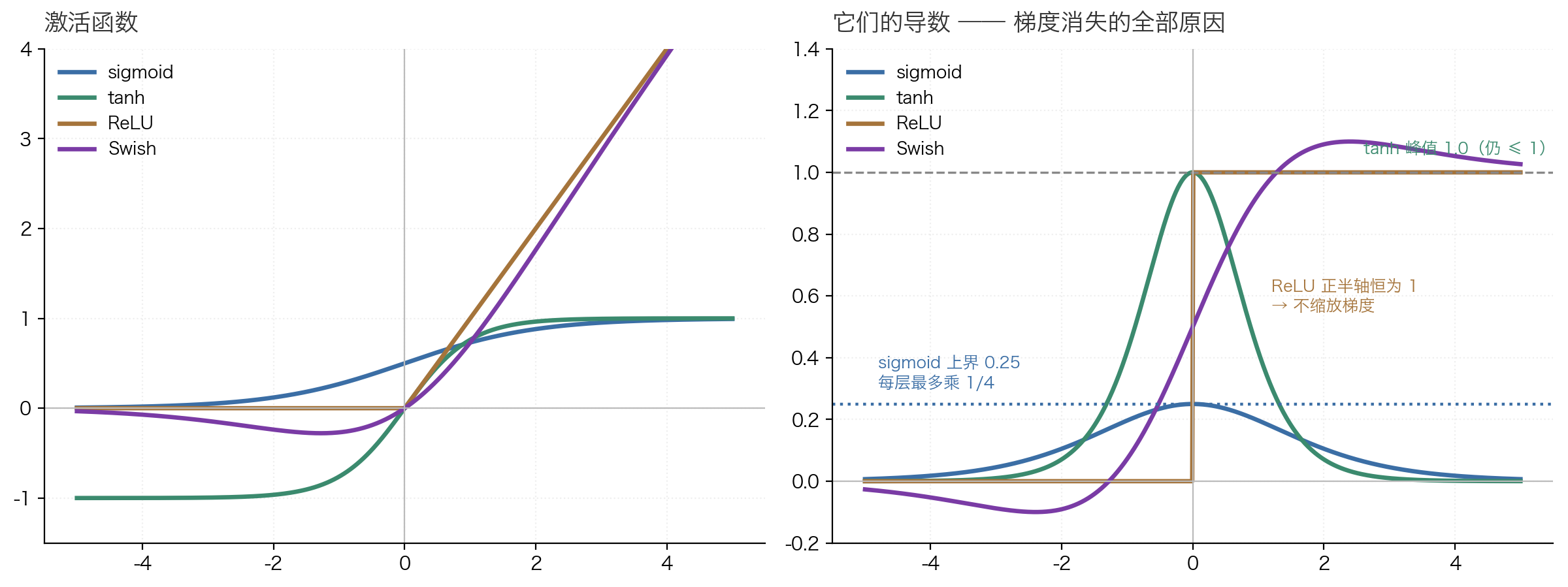 The right-hand panel is the whole section: sigmoid’s derivative is capped at 0.25, so every layer multiplies by at most 1/4; tanh peaks at 1.0 but is still ≤1; only ReLU sits at exactly 1 on the positive side and does not scale the gradient at all.
The key intuition: the derivatives of sigmoid and tanh can only ever shrink the gradient, so vanishing is inevitable once you go deep. ReLU’s derivative is exactly 1 on the positive side, and that is the entire reason it can train deep networks. The price is that it is exactly 0 on the negative side — a neuron whose pre-activation is negative for every input never sees gradient again and dies.
Self-test · A1.2
Q A1.2.1 — Compare sigmoid, tanh and ReLU as hidden-layer activations. Give the failure mode of each.
Sigmoid. Derivative \(\le 0.25\), so every layer multiplies gradient by at most \(1/4\) → vanishing gradients compound with depth. Also not zero-centred, so all gradients into a weight share a sign → zig-zag optimisation. Still correct for output layers producing a probability.
tanh. Zero-centred, fixes the sign problem, derivative peaks at 1. But the factor still only ever shrinks — vanishing is delayed, not solved.
ReLU. Derivative exactly 1 on the positive side, so gradients flow; cheap. Failure mode is dying ReLU: a unit whose pre-activation is negative for every input gets zero gradient forever.
Follow-ups
- Why did the field settle on gated variants? → Empirical. Shazeer’s own paper says they “owe their success to divine benevolence.” There is no clean theory.
Traps
- Calling tanh “the fix for vanishing gradients.” It only raises the cap from 0.25 to 1.
Q A1.2.2 — Why is \(F = \tfrac{8}{3}D\) for SwiGLU instead of \(4D\)?
SwiGLU has three matrices (\(3DF\) parameters) where a vanilla FFN has two (\(2\cdot4D^2=8D^2\)). Setting \(3DF = 8D^2\) gives \(F=\tfrac83 D\) — the parameter count is held constant so the comparison is fair.
Traps
- Writing the FFN with two matrices.
A1.3 Gradients, Jacobians, Hessians
A derivative is a statement about sensitivity: \(\partial f/\partial x = 3\) means that moving \(x\) by \(h\) moves \(f\) by roughly \(3h\).
The gradient \(\nabla f\) is the vector of partial derivatives (scalar output).
The Jacobian (for \(f:\mathbb R^n\to\mathbb R^m\)) is an \(m\times n\) matrix, shaped outputs × inputs:
\[\frac{\partial f}{\partial x}=\begin{bmatrix} \partial f_1/\partial x_1 & \cdots & \partial f_1/\partial x_n\\ \vdots & \ddots & \vdots\\ \partial f_m/\partial x_1 & \cdots & \partial f_m/\partial x_n\end{bmatrix}\]The Hessian is the matrix of second partials \(H_{ij}=\partial^2 f/\partial x_i\partial x_j\). It describes the curvature of the loss surface, and is positive semi-definite at a minimum.
Chain rule: multiply derivatives for scalars, Jacobians for vectors.
\[\frac{\partial \mathbf h}{\partial \mathbf x}=\frac{\partial \mathbf h}{\partial \mathbf z}\frac{\partial \mathbf z}{\partial \mathbf x}\]Why nobody materialises the Hessian for an LLM. It is \(P\times P\). At 70B parameters that is \(5\times10^{21}\) entries. Second-order methods use Hessian-vector products (a second backward pass) or diagonal approximations instead — Adam’s \(v\) is a crude diagonal proxy.
Self-test · A1.3
Q A1.3.1 — What is the Jacobian of softmax, and why is it never materialised?
For one row, \(\partial p_i/\partial s_j = p_i(\delta_{ij}-p_j)\), so the Jacobian is \(\mathrm{diag}(p) - pp^\top\) — a dense \(T\times T\) matrix per row, i.e. \(T^3\) to materialise for a sequence.
The backward pass computes the matrix-vector product directly:
\[dS = P \odot \big(dP - \mathrm{rowsum}(dP \odot P)\big)\]Follow-ups
- Where does this show up? → It is the middle line of the attention backward pass, and interviewers ask about this specific step.
Q A1.3.2 — What does the Hessian tell you, and why is positive semi-definiteness relevant?
Curvature of the loss surface. At a local minimum it is PSD (all eigenvalues \(\ge 0\)), meaning every direction curves upward. The condition number (ratio of largest to smallest eigenvalue) tells you how ill-conditioned the problem is — a high condition number is exactly why plain gradient descent zig-zags and why adaptive methods help.
Follow-ups
- Connection to Adam? → Adam’s \(\sqrt{v}\) is a diagonal approximation to curvature: divide each coordinate by its own recent gradient magnitude, which is a cheap per-coordinate preconditioner.
A1.4 Backpropagation and the computation graph
Two core ideas. If you can explain these two, you can rebuild autograd from scratch:
- Every operation stores a closure that knows how to push gradient back to its own inputs. The graph is built implicitly during the forward pass, each node capturing its parents and its local derivative rule.
- Gradients accumulate, and traversal is in reverse topological order. A node used in several places receives gradient along several paths — hence
+=rather than=. The topological sort guarantees that when you call a node’s backward, all of its consumers have already contributed.
def backward(self):
    topo, seen = [], set()
    def build(v):
        if v in seen: return
        seen.add(v)
        for c in v._prev: build(c)
        topo.append(v)
    build(self)
    self.grad = 1.0
    for v in reversed(topo):     # reverse topological order
        v._backward()
Why backward is roughly 2× the forward in compute. Each layer needs two matmuls: \(\partial L/\partial X\) (passed upstream) and \(\partial L/\partial W\) (used to update this layer). So forward + backward ≈ 3× forward, or 4× with gradient checkpointing.
Self-test · A1.4
Q A1.4.1 — In a from-scratch autograd, why is it self.grad += ... rather than =?
Because a node can be used more than once in the graph. It receives gradient from every consumer, and = would silently discard all but the last. This single character is the most common bug when people write micrograd from memory, and it only shows up on expressions with reused subterms — which is why the test should use one.
Follow-ups
- Why reverse topological order? → It guarantees that when you call a node’s
_backward, every consumer of that node has already contributed its share.- Why does PyTorch accumulate into
.gradby default? → Same reason, plus it makes gradient accumulation across micro-batches free. It is also why you must callzero_grad().
Q A1.4.2 — Why is the backward pass roughly 2× the forward in FLOPs?
Each layer needs two matmuls of the same size as the forward one:
\(\frac{\partial L}{\partial X} = \frac{\partial L}{\partial Z}W^\top \quad\text{(pass upstream)}\) \(\frac{\partial L}{\partial W} = X^\top\frac{\partial L}{\partial Z}\quad\text{(update this layer)}\)
Hence forward + backward \(\approx 3\times\) forward. This is where \(6ND\) comes from: \(2N\) per token forward, \(4N\) backward.
A1.5 Optimizers
SGD \(\theta \leftarrow \theta - \alpha g\). Simple, but it oscillates back and forth on ill-conditioned curvature (large condition number).
Momentum accumulates the history of gradient directions, damping oscillation and accelerating consistent directions:
\[v_t=\beta v_{t-1}+g_t,\qquad \theta_t=\theta_{t-1}-\alpha v_t\]Adam maintains a first moment (direction) and a second moment (per-coordinate step size):
\[m_t = \beta_1 m_{t-1}+(1-\beta_1)g_t,\qquad v_t = \beta_2 v_{t-1}+(1-\beta_2)g_t^2\] \[\hat m_t=\frac{m_t}{1-\beta_1^t},\quad \hat v_t=\frac{v_t}{1-\beta_2^t},\qquad \theta_t=\theta_{t-1}-\alpha\frac{\hat m_t}{\sqrt{\hat v_t}+\epsilon}\]Bias correction exists because \(m_0=v_0=0\), which biases the early estimates toward zero.
AdamW takes weight decay out of the gradient and applies it directly to the weights:
\[\theta_t=\theta_{t-1}-\alpha\frac{\hat m_t}{\sqrt{\hat v_t}+\epsilon}-\alpha\lambda\theta_{t-1}\]The memory bill. Adam keeps two fp32 states per parameter = 8 bytes, which is half of the 16 bytes/parameter budget of mixed-precision training. That is the entire reason ZeRO exists.
Typical LLM hyperparameters: \(\beta_1=0.9\), \(\beta_2=0.95\) (below the 0.999 default, because a long-horizon second moment goes stale), weight decay 0.1.
Self-test · A1.5
Q A1.5.1 — What exactly does AdamW change relative to Adam, and why does it matter?
In Adam, L2 regularisation is added to the gradient, so it then passes through the same adaptive scaling as everything else. The effective decay ends up inversely proportional to the gradient’s recent magnitude — parameters with small gradients get decayed hard, parameters with large gradients barely at all. That is not what anyone means by weight decay.
AdamW applies the decay directly to the weights, outside the adaptive step, restoring the intended uniform pull toward zero.
Follow-ups
- Anything newer? → Muon orthogonalises the momentum update for 2D parameters via Newton-Schulz iteration, with reported gains at LLM scale.
Traps
- Saying AdamW “is just Adam with weight decay.” Adam can have decay too; the difference is where it goes.
Q A1.5.2 — Why does Adam need bias correction?
\(m_0 = v_0 = 0\), so early estimates are biased toward zero — at step 1, \(m_1 = (1-\beta_1)g_1\), which is only 10% of the true gradient with \(\beta_1=0.9\). Dividing by \(1-\beta_1^t\) corrects this, and the correction decays to 1 as \(t\) grows.
Follow-ups
- What happens without it? → Tiny steps for the first few hundred iterations. Interacts with warmup: both address early-training instability, from different directions.
A1.6 Learning rate schedules
Warmup. Over the first few hundred steps Adam’s \(\hat v\) is built from too few samples and is noisy, so the adaptive denominator is unreliable and the effective step can be enormous. Warmup keeps the steps small until the estimate stabilises. Typically 1–2% of total steps.
Cosine decay. Big steps early to get through bad regions fast, small steps late to converge. Cosine rather than linear or stepwise is mostly an empirical finding.
A constraint that bites. Cosine is defined against a fixed total step count. If you decide halfway through that you want to train longer, you cannot simply extend it — the learning rate has already decayed. This is exactly why WSD (warmup-stable-decay) became popular: you can branch a decay phase off the constant segment at any point, which turns midtraining and continued pretraining into repeatable operations rather than decisions welded shut before the run starts.
Self-test · A1.6
Q A1.6.1 — Why warmup? Does pre-LN remove the need for it?
Warmup exists because Adam’s second-moment estimate is unreliable early, so the effective step can be enormous.
Pre-LN reduces the architectural need (post-LN puts a normalisation on the residual path, so gradients get rescaled every layer and deep models need careful warmup). But the optimizer-state argument still stands, so runs still use warmup.
Q A1.6.2 — Why has WSD become popular over cosine?
Cosine is defined against a fixed total step count, so the schedule commits you at step 0. WSD keeps a constant “stable” phase from which you can branch a decay at any point — which makes midtraining, continued pretraining, and “train longer if it is still improving” all practical.
Follow-ups
- Why does the decay phase matter so much? → Data seen during the final decay has outsized influence on the final weights. That is why you save your best data for last.
A1.7 Normalisation
Why not BatchNorm (three reasons — give more than one in an interview):
- sequence lengths vary, so batch statistics are computed over a ragged set of positions;
- batch statistics couple the examples in a batch, which breaks batch-1 autoregressive generation;
- under distributed training every forward pass needs a cross-device synchronisation.
LayerNorm normalises inside a single token’s feature vector, independent of batch composition:
\[\text{LN}(x)=\gamma\odot\frac{x-\mu}{\sqrt{\sigma^2+\epsilon}}+\beta\]RMSNorm drops the mean subtraction and the bias:
\[\text{RMSNorm}(x)=\gamma\odot\frac{x}{\sqrt{\tfrac1D\sum_i x_i^2+\epsilon}}\]Ablations show that re-scaling is what does the work and re-centring contributes essentially nothing, and dropping it removes one reduction over the feature dimension — which matters when it is two per layer across 80 layers.
What \(\gamma\) is for. Normalisation forces unit RMS, which destroys learned scale information. \(\gamma\) hands per-dimension magnitude control back: \(\gamma_i>1\) amplifies, \(\gamma_i\approx 0\) kills that dimension.
Pre-LN vs post-LN. Pre-LN normalises the sublayer input, so the residual stream stays a clean identity path and the architectural need for warmup goes away. The cost is that the residual stream grows in magnitude with depth, so you need a final norm before the output head.
Self-test · A1.7
Q A1.7.1 — Give three reasons transformers use LayerNorm rather than BatchNorm.
Variable sequence length; coupling of examples in a batch (breaks batch-1 generation); and cross-device synchronisation in distributed training. See above for the full form.
Traps
- Giving only one reason. Give three.
Q A1.7.2 — Under bf16, what part of RMSNorm must stay in fp32, and why?
The reduction — the mean-square over the feature dimension. Summing \(D\) squared values in bf16 accumulates rounding error badly. Compute in fp32 and cast the result back, which is why implementations end with .type_as(x).
Follow-ups
- What else must stay fp32? → Softmax denominators, loss accumulation, gradient all-reduce. The rule is: reductions in fp32, elementwise ops in low precision.
A1.8 Generalisation, regularisation and double descent
Bias-variance decomposition (squared loss):
\[\mathbb E[(y-\hat f)^2]=\underbrace{(\mathbb E[\hat f]-f)^2}_{\text{bias}^2}+\underbrace{\operatorname{Var}[\hat f]}_{\text{variance}}+\sigma^2\]The classical picture: capacity ↑ → bias ↓, variance ↑ → a U-shaped test error, and you take the bottom.
Why that is no longer the whole story for LLMs. Modern networks are trained far past the interpolation threshold (zero training error) and test error keeps falling — double descent. The classical U-curve is only the first descent; there is a second one after the interpolation point. So “bigger models overfit more” is simply not what is observed at LLM scale.
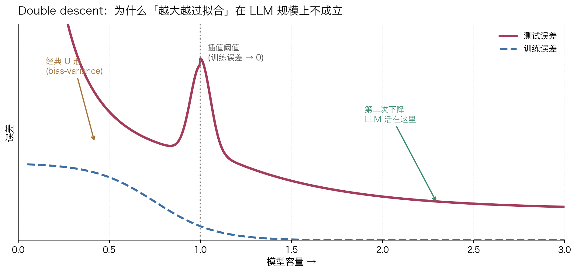 The classical U-curve is only the first descent. Past the interpolation threshold test error falls again — and LLMs all live on the right-hand side.
The honest statement is that the decomposition is still correct but no longer predictive, because the implicit regularisation coming from SGD and the architecture is doing work the framework never modelled.
The regularisation that actually operates in LLM pretraining is mostly data scale and weight decay. Dropout has essentially disappeared from pretraining (it hurts when data is plentiful).
Self-test · A1.8
Q A1.8.1 — Does bias-variance explain why bigger LLMs are better?
No — the classical U-curve predicts the opposite. What is observed is double descent: past the interpolation threshold, test error falls again. The decomposition is still correct but not predictive, because implicit regularisation from SGD and architecture is doing unmodelled work.
Follow-ups
- Do LLMs overfit at all? → Yes, on repeated data. The reason pretraining rarely overfits is that it is close to single-epoch on a corpus larger than the model can memorise.
Q A1.8.2 — Why has dropout largely disappeared from LLM pretraining?
Dropout is a regulariser for the data-scarce regime. Pretraining is data-rich and close to single-epoch, so there is little overfitting to prevent — and dropout costs capacity and throughput. It still appears in fine-tuning on small datasets.
Follow-ups
- What is inverted dropout? → Scale by \(1/(1-p)\) at train time so that inference needs no rescaling. This is what every framework does, and it is why
model.eval()can simply disable it.
A1.9 Loss functions and information theory
\[\operatorname{CE}(p,q)=-\sum_x p(x)\log q(x),\qquad \operatorname{KL}(p\,\|\,q)=\sum_x p(x)\log\frac{p(x)}{q(x)},\qquad H(p)=-\sum_x p(x)\log p(x)\]How the three relate (two lines to prove):
\[\operatorname{CE}(p,q)=\operatorname{KL}(p\,\|\,q)+H(p)\]What this means for LM training. The target is one-hot, so \(H(p)=0\) and cross-entropy is the KL divergence; it also reduces to the negative log-likelihood of the next token:
\[\mathcal L=-\sum_{t=1}^{T}\log p(x_t\mid x_{<t})\]forward vs reverse KL — the single most classic question here, and the difference is entirely about which side the infinite penalty sits on:
| Weighted by | Behaviour | Where it is used | |
|---|---|---|---|
| Forward \(\operatorname{KL}(p|q)\) | \(p\) | mean-covering: \(q\) must cover all of \(p\)’s support, smearing across modes | Maximum likelihood |
| Reverse \(\operatorname{KL}(q|p)\) | \(q\) | mode-seeking: ignoring a mode is unpunished, so it collapses onto one | Variational inference, the KL penalty in RLHF |
Self-test · A1.9
Q A1.9.1 — Prove \(\operatorname{CE}(p,q) = \operatorname{KL}(p\|q) + H(p)\).
\[\operatorname{KL}(p\,\|\,q) = \sum_x p(x)\log p(x) - \sum_x p(x)\log q(x) = -H(p) + \operatorname{CE}(p,q)\]Rearrange. Two lines.
Follow-ups
- Is KL a distance? → No. Not symmetric, no triangle inequality.
Q A1.9.2 — Why is forward KL mean-covering and reverse KL mode-seeking?
Forward KL weights by \(p\), so wherever \(p\) has mass and \(q\) does not, \(\log(p/q)\to\infty\) and you pay enormously — \(q\) is forced to cover all of \(p\)’s support, smearing across modes.
Reverse KL weights by \(q\), so \(q\) is punished for putting mass where \(p\) has none, but pays nothing for ignoring a mode entirely (those regions have \(q\approx0\), so they contribute \(\approx 0\) to the sum). It therefore collapses onto one mode and does it well.
Traps
- Getting them backwards. This is the question Sapora says she answered wrong and cried about afterwards — and she had handled it in two of her own papers. Rehearse the things you already know.
A1.10 Numerical stability
Three things to watch: \(e^x\) overflows for large \(x\) (around \(x\approx89\) in fp32); \(\log x\) underflows for \(x\) near 0; and \(\log x\) loses precision for \(x\) near 1.
softmax exploits shift invariance:
\[\text{softmax}(x)_i=\frac{e^{x_i-c}e^c}{\sum_j e^{x_j-c}e^c}=\text{softmax}(x-c)_i\]Take \(c=x_\max\) and the largest exponential becomes \(e^0=1\).
log-softmax should never be written as log(softmax(x)) (taking the log of small probabilities is unstable). Use
logsumexp uses the same trick: \(\log\sum_i e^{x_i}=x_\max+\log\sum_i e^{x_i-x_\max}\)
The same recurrence shows up again. FlashAttention’s online softmax carries a running max and rescales each block by \(e^{m_\text{old}-m_\text{new}}\) — this very shift invariance, applied incrementally.
Self-test · A1.10
Q A1.10.1 — Why does F.cross_entropy take logits rather than probabilities?
So it can use the numerically stable path internally: logits → logsumexp → gather, never an explicit softmax followed by a log. Passing probabilities forces the unstable log(p) for small \(p\), and also loses the max-subtraction trick.
Traps
- Writing
torch.log(torch.softmax(x)). Always uselog_softmax.
A1.11 The training loop and debugging
for batch in loader:
    optimizer.zero_grad()                                     # 1
    logits = model(batch.input_ids)                           # 2
    loss = F.cross_entropy(
        logits[:, :-1].reshape(-1, V),                        # 3  shift
        batch.labels[:, 1:].reshape(-1),
        ignore_index=-100)                                    # 4  mask
    loss.backward()                                           # 5
    torch.nn.utils.clip_grad_norm_(model.parameters(), 1.0)   # 6
    optimizer.step()                                          # 7
    scheduler.step()                                          # 8
Three bugs that really happen:
- Forgetting
zero_grad(). PyTorch accumulates gradients by default. Without it you are effectively training on an ever-growing batch of stale gradients. The loss slowly goes strange and it is hard to catch. - Off-by-one in the shift. Position \(t\) must predict token \(t+1\). Get it wrong and either the model sees the answer (suspiciously fast loss) or it is asked to predict out of nothing.
- Forgetting the loss mask. Computing loss on prompt tokens during SFT, or on padding. This never crashes; it silently degrades quality.
The debugging move worth volunteering: overfit ten examples first. If the model cannot even memorise ten examples, the bug is in the code, not in the hyperparameters. This single test isolates the large majority of the problems above.
What actually causes exploding gradients in practice (not depth — pre-LN plus residuals took care of that): a bad batch of data, a learning rate too high for the current curvature, fp16 overflow. Mitigations: global gradient-norm clipping (and log the pre-clip norm — its spikes are the earliest warning), bf16, warmup. If you are clipping often, clipping is masking a problem.
Self-test · A1.11
Q A1.11.1 — Walk through one training step and name the three most common bugs.
See the loop above. The three: missing zero_grad(); off-by-one in the label shift; missing loss mask on prompt or padding tokens.
Follow-ups
- Where does gradient accumulation go? → Skip
zero_grad/stepfor \(k\) micro-batches and divide the loss by \(k\).- Why clip before
step()? → The optimizer consumes.grad; clipping after would do nothing.
Q A1.11.2 — Your loss is not decreasing. What do you check, in order?
- Overfit ten examples. If that fails, the bug is in the code. This is the single highest-value test and it isolates most causes.
- Is
zero_grad()called? Is the model intrain()mode? - Are labels shifted correctly? Is the mask right?
- Is the learning rate sane after warmup — print the actual value, not the config.
- Are gradients reaching all parameters? Check for
Nonegrads and for anything detaching the graph. - Is the data actually shuffled, and is the loader returning what you think?
Follow-ups
- Loss is NaN, not flat — different checklist? → Yes: check for inf in the input, division by zero,
log(0), fp16 overflow, and a learning rate that is simply too high.
A1.12 Basic statistics
Only a small handful of these actually recur in interviews.
Expectation and variance
\[\mathbb E[aX+b]=a\mathbb E[X]+b,\qquad \operatorname{Var}[aX+b]=a^2\operatorname{Var}[X]\] \[\operatorname{Var}[X]=\mathbb E[X^2]-\mathbb E[X]^2\]Linearity of expectation holds for any random variables and does not need independence — which is what makes it so useful as a proof tool. Additivity of variance does need independence (or at least uncorrelatedness).
\[\mathbb E\Big[\sum_i X_i\Big]=\sum_i\mathbb E[X_i]\quad\text{(always)}\] \[\operatorname{Var}\Big[\sum_i X_i\Big]=\sum_i\operatorname{Var}[X_i]\quad\text{(needs independence)}\]Common distributions
| Distribution | \(\mathbb E\) | \(\operatorname{Var}\) | Where it shows up |
|---|---|---|---|
| Bernoulli(\(p\)) | \(p\) | \(p(1-p)\) | Binary rewards, pass/fail |
| Binomial(\(n,p\)) | \(np\) | \(np(1-p)\) | Number of successes in \(n\) samples |
| Geometric(\(p\)) | \(1/p\) | \((1-p)/p^2\) | Samples until the first success (best-of-N) |
| Gaussian(\(\mu,\sigma^2\)) | \(\mu\) | \(\sigma^2\) | Initialisation, noise |
A trick that keeps coming back: squaring an indicator. For a binary variable \(X\in\{0,1\}\), \(X^2=X\), so \(\mathbb E[X^2]=\mathbb E[X]=p\) and therefore \(\operatorname{Var}=p-p^2=p(1-p)\).
Why this one matters in RL. The variance of a binary reward is \(\hat p(1-\hat p)\): maximal at \(\hat p=0.5\) and zero at both ends. That is the mathematical source of the fact that tasks the model always gets right and tasks it always gets wrong both produce no gradient (see A12.3).
Self-test · A1.12
Q A1.12.1 — A model solves a task with probability \(p\). You sample \(n\) times and take best-of-\(n\). What is the probability of at least one success, and what is the expected number of samples until the first success?
At least one success: \(1-(1-p)^n\). Expected samples until first success: \(1/p\) (geometric).
For \(p = 0.1\): best-of-10 succeeds with probability \(1-0.9^{10} = 65\%\), and you would expect to need 10 samples for the first success. This is the arithmetic behind test-time scaling — and it also shows the diminishing returns, since going from \(n=10\) to \(n=100\) only moves you from 65% to 99.997%.
Follow-ups
- Why does best-of-\(n\) need a verifier? → Without one you cannot tell which of the \(n\) samples succeeded, so the probability is irrelevant. The bottleneck for test-time scaling is almost always ranking, not sampling.
A1.13 Gradient flow through sampling
The problem. You want to backpropagate through a discrete sample, but \(z\sim\text{Categorical}(p_\theta)\) is not differentiable — sampling severs the gradient. This comes up in MoE routing, discrete latents, and anywhere else you have to “pick one.”
Three ways around it:
1. REINFORCE / score function estimator (the policy gradient of A4.2)
\[\nabla_\theta\mathbb E_{z\sim p_\theta}[f(z)]=\mathbb E_{z\sim p_\theta}\big[f(z)\nabla_\theta\log p_\theta(z)\big]\]Unbiased, but high variance. It applies when \(f\) is non-differentiable or even a black box (say \(f\) is a verifier).
2. The reparameterization trick
Move the randomness onto a noise source that does not depend on the parameters. For a Gaussian:
\[z=\mu_\theta+\sigma_\theta\odot\epsilon,\qquad \epsilon\sim\mathcal N(0,I)\]Now \(z\) is differentiable in \(\theta\). Far lower variance, but it only works for continuous distributions — which is why VAEs can be trained this way.
3. Gumbel-Softmax / Concrete
A continuous relaxation of a discrete variable. Add Gumbel noise to the logits and take a softmax at temperature \(\tau\):
\[y_i=\frac{\exp((\log p_i+g_i)/\tau)}{\sum_j\exp((\log p_j+g_j)/\tau)},\qquad g_i\sim\text{Gumbel}(0,1)\]As \(\tau\to0\) it approaches one-hot sampling; at large \(\tau\) it is smooth and differentiable. Biased but low variance.
Straight-through estimator (STE). Forward uses a hard argmax (so the output stays discrete); backward pretends it was the identity (or uses the softmax’s gradient). This is exactly how quantization-aware training (QAT) pushes gradient through the rounding operation.
One-line selection guide. \(f\) non-differentiable or a black box → REINFORCE; continuous distribution → reparameterization; discrete distribution you can relax → Gumbel-Softmax or STE.
Self-test · A1.13
Q A1.13.1 — Why can’t you use the reparameterization trick for a categorical distribution?
Reparameterization requires expressing the sample as a differentiable function of the parameters and a parameter-free noise source. For a categorical, the sample is a discrete index — any such expression involves an argmax or a step function, whose derivative is zero almost everywhere and undefined at the jumps. There is no smooth path from \(\theta\) to the sampled index.
Gumbel-Softmax works around this by relaxing the output: instead of an index it returns a near-one-hot continuous vector, which is differentiable. You pay a bias for it.
Follow-ups
- Where does STE show up in LLM work? → Quantization-aware training: forward rounds to INT8, backward passes gradient through as if it were identity. Also in some MoE routers.
- Is REINFORCE ever preferred despite the variance? → Yes, whenever the reward is a black box — a unit test, a compiler, a human. That is exactly the RLHF/RLVR setting.
A1.14 The bits of theoretical CS that come up
The theoretical CS that shows up in ML interviews is narrow — basically just these.
Complexity notation. \(O\) is an upper bound, \(\Omega\) a lower bound, \(\Theta\) a tight bound. Note that attention is \(O(n^2 d)\) — saying \(O(n^2)\) hides the \(d\), which is fine at long context but misleading when you compare different \(d\).
Amortised analysis. A single push onto a dynamic array is \(O(n)\) in the worst case but \(O(1)\) amortised. Paged allocation of the KV cache is the same idea: an individual growth step allocates a new block, but amortised it is constant.
Dynamic programming = memoisation + optimal substructure. Beam search is not DP (it is a greedy approximation); Viterbi is.
Divide and conquer, and the master theorem. \(T(n)=aT(n/b)+f(n)\). In collective communication it applies to recursive halving/doubling and to tree all-reduce, where each step halves the problem.
Note that ring all-reduce does not belong to this family — it is a linear pipeline, not divide and conquer, and the master theorem does not apply. Just count directly: \(2(p-1)\) steps, each moving \(N/p\), so every device sends and receives \(2N(p-1)/p\approx 2N\), almost independent of the device count, which is the entire reason it scales.
Self-test · A1.14
Q A1.14.1 — Why is ring all-reduce bandwidth-optimal?
Each device sends and receives \(2N(p-1)/p\) bytes total, which tends to \(2N\) as \(p\) grows — independent of the number of devices. The lower bound for all-reduce is \(2N(p-1)/p\), so ring achieves it.
The cost is latency: it takes \(2(p-1)\) sequential steps, so with many small tensors the per-step overhead dominates. That is why frameworks bucket gradients into large flat buffers before all-reducing, and why tree-based algorithms are used for small messages.
Follow-ups
- Why does that matter for ZeRO? → all-reduce = reduce-scatter + all-gather, each \(N(p-1)/p\). So ZeRO-2 costs the same total bandwidth as DDP while storing \(1/p\) of the state. ZeRO-3 adds one more all-gather, so ~1.5× DDP’s communication.
Concepts still to add: MLE and MAP; weight initialisation (Xavier / Kaiming / why LLMs use \(\mathcal N(0,0.02)\)); gradient checkpointing; classical models (logistic regression / decision trees / k-means / SVM).
A2 · Transformer architecture and implementation
This section is where the coding round lives: causal self-attention gets asked six different ways. Alisa’s book is deepest here, but she does not cover MoE, tokenization, multimodality or SSMs at all — those are additions (marked ★).
How to read it: A2.1–A2.4 are the skeleton and you must be able to rebuild them closed-book; A2.5–A2.8 are the choices every modern model makes; A2.9–A2.13 are what you reach for to show depth when pushed.
A2.1 The three architectural paradigms
Lay the map out before talking about attention, otherwise none of the later “why” questions have a frame of reference.
| Attention | Training objective | Good at | |
|---|---|---|---|
| Encoder-only (BERT) | Bidirectional | Masked LM | Classification, retrieval, embeddings |
| Decoder-only (GPT) | Causal | Next-token | Generation, plus everything else reachable by prompting |
| Encoder-decoder (T5) | Enc bidirectional, Dec causal + cross | Seq2seq | Translation, genuine sequence-to-sequence |
Three reasons decoder-only won:
- Training efficiency. Every position is one supervised prediction. MLM masks only ~15%, so for the same amount of data you get roughly 6× less signal.
- Architectural simplicity. One stack, no cross-attention, easier to scale and to shard.
- In-context learning. Prompting turns almost every task into generation, so no task-specific heads.
Bidirectional attention still owns a domain: embeddings and retrieval. There you encode a fixed input and want every token to see the whole text. Modern embedding models often start from a decoder-only model, remove the causal mask, and keep training.
Self-test · A2.1
Q A2.1.1 — Why did decoder-only win, and where is it still the wrong choice?
Three reasons it won: signal density (every position supervised, versus ~15% for MLM), architectural simplicity (one stack, no cross-attention, easier to shard), and in-context learning (prompting removes the need for task heads).
Where it is wrong: embedding and retrieval, where you encode a fixed input and want bidirectional context. Also genuine seq2seq with a long fixed source, where an encoder-decoder can encode the source once and cross-attend to it repeatedly.
Follow-ups
- What is cross-attention? → Q from the decoder, K/V from the encoder output. A decoder-only model has none — its “context” is just earlier positions in the same sequence.
Traps
- Answering only “decoder-only is simpler.” The training-signal-density argument is far stronger.
A2.2 Anatomy of a block: the residual stream
A transformer block is only two lines:
x = x + self.attn(self.norm1(x))     # pre-norm, residual
x = x + self.mlp(self.norm2(x))
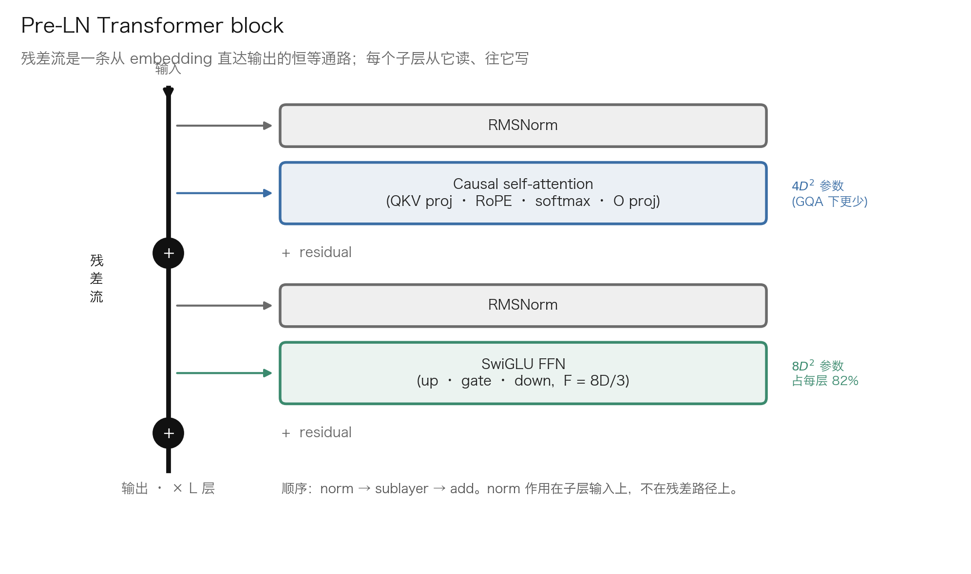
The residual-stream view is the single most useful mental model for the whole architecture: treat \(x\) as a shared bus running from the embedding all the way to the output. Every layer reads from the bus, computes something, and writes back to it.
That view immediately explains several things:
- A useless layer learns to write approximately zero, without having to learn the identity map — which is the real value of a residual connection.
- A 100-layer network behaves more like “an ensemble of many short paths” than like one 100-layer-deep path.
- Layers communicate through the bus, so it makes sense to say “this layer wrote that feature into the stream.”
Pre-LN vs post-LN.
- Post-LN (the original paper): \(x \leftarrow \text{LN}(x + \text{sublayer}(x))\). The normalisation sits on the residual path, gradients get rescaled at every layer, and deep models will not train without a carefully tuned warmup.
- Pre-LN: \(x \leftarrow x + \text{sublayer}(\text{LN}(x))\). The residual stream is a clean identity path from embedding to output. Xiong et al. showed this is exactly why warmup can be dropped.
The cost of pre-LN (be sure you can state it): the residual stream grows in magnitude with depth, so a final norm before the output head is mandatory; very deep pre-LN models can also show representation collapse in their later layers — which is what variants like sandwich norm exist for.
Self-test · A2.2
Q A2.2.1 — Why did the field switch from post-LN to pre-LN, and what did it cost?
Post-LN puts the normalisation on the residual path, so gradients are rescaled at every layer and deep models need a carefully tuned warmup to train at all. Pre-LN leaves a clean identity path from embedding to output, which is what removes the warmup requirement.
The cost: the residual stream grows in magnitude with depth, since every layer adds to it and nothing rescales it. You need a final norm before lm_head. Very deep pre-LN models can also show representation collapse in later layers, which is what sandwich norm (normalising both before and after the sublayer) addresses.
Traps
- Praising pre-LN without naming the cost. You will get pushed on it.
- Forgetting that final norm when writing a model from scratch.
A2.3 Self-attention and \(\sqrt{d_k}\)
\[\text{Attn}(Q,K,V) = \text{softmax}\!\left(\frac{QK^\top}{\sqrt{d_k}} + M\right)V\]The argument for the scaling factor (three steps, memorise them): take \(q,k\) with independent, unit-variance components. The dot product is a sum of \(d_k\) such products, so
\[\operatorname{Var}[q\cdot k] = d_k,\qquad \text{std} = \sqrt{d_k}\]At \(d_k = 128\) the logits already span roughly \(\pm 11\) before training has started. A softmax over a range that wide is nearly one-hot, and a saturated softmax has vanishing gradients — the attention pattern is frozen at initialisation and cannot learn. Dividing by \(\sqrt{d_k}\) pulls the variance back to 1.
Why \(d_k\) and not \(d_\text{model}\). The dot product is taken over the head dimension, and that is the dimension whose variance you need to fix. Get it wrong and the model still trains, just worse — which is exactly what makes it a good exam question.
The causal mask is applied additively as \(-\infty\) before the softmax. Multiplying by 0 is wrong: the masked positions still enter the denominator, so the surviving weights no longer sum to 1.
Self-test · A2.3
Q A2.3.1 — Explain the scaling factor. What breaks without it?
Logits have standard deviation \(\sqrt{d_k}\) at initialisation, so with \(d_k=128\) they span roughly \(\pm 11\) before any training. Softmax over logits that wide is nearly one-hot, and a saturated softmax has vanishing gradients — the attention pattern is frozen at init and cannot learn.
Dividing by \(\sqrt{d_k}\) restores unit variance. It is the same knob as softmax temperature: \(1/\sqrt{d_k}\) is a temperature chosen to keep attention entropy reasonable at initialisation.
Follow-ups
- When does the argument stop holding? → It assumes the initialisation it describes. Once weights drift, logits can grow again — which is exactly what QK-normalisation (RMSNorm on Q and K before the dot product) was introduced to handle at large scale.
Traps
- Using \(\sqrt{d_\text{model}}\).
- Saying only “it normalises,” without the variance magnitude and the softmax-saturation steps.
Q A2.3.2 — Why is the causal mask additive before softmax rather than multiplicative after?
Because softmax normalises over the whole row. If you zero out masked positions after the softmax, those positions still contributed to the denominator, so the surviving weights no longer sum to 1 — every row is silently scaled down by the masked fraction, and the scaling differs by position.
Adding \(-\infty\) before the softmax makes \(e^{-\infty}=0\) contribute nothing to the denominator, so the remaining weights are a proper distribution.
A2.4 Writing it from scratch
class CausalSelfAttention(nn.Module):
    def __init__(self, d_model, n_heads, max_len=512, dropout=0.0):
        super().__init__()
        assert d_model % n_heads == 0
        self.n_heads, self.d_head = n_heads, d_model // n_heads
        self.qkv  = nn.Linear(d_model, 3 * d_model, bias=False)
        self.proj = nn.Linear(d_model, d_model, bias=False)
        self.attn_drop, self.resid_drop = nn.Dropout(dropout), nn.Dropout(dropout)
        self.register_buffer("mask",
            torch.tril(torch.ones(max_len, max_len)).view(1, 1, max_len, max_len))

    def forward(self, x):
        B, T, C = x.shape
        q, k, v = self.qkv(x).split(C, dim=2)
        q = q.view(B, T, self.n_heads, self.d_head).transpose(1, 2)   # (B, nh, T, hd)
        k = k.view(B, T, self.n_heads, self.d_head).transpose(1, 2)
        v = v.view(B, T, self.n_heads, self.d_head).transpose(1, 2)

        att = (q @ k.transpose(-2, -1)) / math.sqrt(self.d_head)
        att = att.masked_fill(self.mask[:, :, :T, :T] == 0, float("-inf"))
        att = self.attn_drop(F.softmax(att, dim=-1))

        y = (att @ v).transpose(1, 2).contiguous().view(B, T, C)
        return self.resid_drop(self.proj(y))
Four traps, all inside these twenty lines:
-
.contiguous()— aftertransposeyou hold a view with non-contiguous strides, and.view()raises..reshape()also works (copying when it must), but be able to state the difference. - Divide by
sqrt(d_head), notsqrt(d_model). - Additive
-infmask before the softmax (reason in A2.3). - Fuse QKV into one projection. Three
nn.Linearcalls are mathematically equivalent but slower — at identical FLOPs, one GEMM beats three.
Shape discipline. Encode shapes in the variable names (Shazeer’s shape-suffix convention): x_BTC, q_BHTD. In a setting whose failure mode is a silent transpose, the bug then surfaces at the call site instead of three lines later.
Mask convention. tensor.masked_fill(mask, value) fills the positions where the mask is True. So if your mask uses True to mean allowed, you need masked_fill(~mask, -inf). Half of all mask bugs are this inversion.
Three lines that verify causality (and double as a debugging tool):
y1 = model(x)
x2 = x.clone(); x2[:, -1, :] += 10.0
assert torch.allclose(y1[:, :-1], model(x2)[:, :-1])   # the past cannot see the future
Self-test · A2.4
Q A2.4.1 — Write multi-head causal self-attention from scratch. No nn.MultiheadAttention.
(Code above.) The four things being checked: .contiguous() after transpose, scaling by \(\sqrt{d_\text{head}}\) not \(\sqrt{d_\text{model}}\), additive \(-\infty\) mask before softmax, and fusing QKV into one projection.
Then say the causality check out loud — perturb the last token, assert earlier outputs are unchanged. Offering the test before being asked is a strong signal.
Follow-ups
register_buffervsnn.Parameter? → A buffer moves with.to(device)and is saved in the state dict, but receives no gradient.- Where does dropout go? → After the attention softmax, and on the residual branch output. Almost always 0 in modern pretraining.
- view vs reshape? →
viewrequires contiguous memory and never copies;reshapefalls back to a copy when it must.
A2.5 Attention variants: MHA → MQA → GQA → MLA
There is one driver and one only: KV cache size — \(2LKH\) elements per token, times the bytes per element.
| Variant | KV heads | Cache (70B, bf16) | Trade-off |
|---|---|---|---|
| MHA | \(N\) = 64 | 2,560 KiB/token | Best quality, cache is unaffordable |
| MQA | 1 | 40 KiB/token | 64× cheaper, measurable quality loss |
| GQA | 8 | 320 KiB/token | 8× cheaper, negligible loss |
| MLA | latent 512+64 | 90 KiB/token | DeepSeek reports it better than MHA |
GQA groups the query heads and shares one K/V head within each group. The implementation is one line: k.repeat_interleave(n_rep, dim=1).
Why GQA beat MQA. MQA keeps a single shared KV head, which is too narrow a bottleneck: quality drops and training is less stable. GQA gives you a tunable knob that captures most of the benefit.
Why DeepSeek chose MLA. In their ablations GQA is slightly worse than MHA while MLA is slightly better — the rare optimisation that is not a trade-off. MLA compresses K/V into a low-rank latent and caches that, plus a small decoupled RoPE key.
Self-test · A2.5
Q A2.5.1 — Walk me through the attention variants. What does each trade, and why did GQA win?
Frame it around one driver: KV cache size, which is \(2LKH\) elements per token — so \(2LKH\times2\) bytes in bf16 — and is what limits concurrency and context length. Everything else is a consequence.
MHA gives every query head its own K/V — best quality, and 2,560 KiB/token for a 70B model, which is unaffordable at long context. MQA collapses to a single shared KV head, a 64× cut, but the bottleneck is too tight: measurable quality loss and less stable training. GQA groups query heads so each group shares one K/V head — 8× with negligible loss, and crucially it is a tunable knob rather than an all-or-nothing choice. That tunability is why it won.
MLA takes a different axis: instead of sharing K/V, project them into a low-rank latent and reconstruct per head, plus a small decoupled RoPE key. Every head keeps its own K/V, just derived from a shared compressed representation. DeepSeek’s ablations show it slightly better than MHA, not merely cheaper — the rare optimisation that is not a trade-off.
Q A2.5.2 — Does GQA reduce FLOPs?
Not the attention computation. K/V are expanded back to \(N\) heads before the matmuls, so the \(QK^\top\) and \(AV\) FLOPs are identical. (Be precise if pushed: the K/V projections do shrink, from \(2D^2\) to \(2DKH\) per layer — real, but a small share of the total.) What GQA buys is memory and bandwidth — the KV cache shrinks by the group factor, and since decoding is memory-bandwidth-bound, that translates into throughput.
This distinction trips people up constantly, and getting it right is a clear signal that you have thought about where decode time actually goes.
Follow-ups
- How do you convert an MHA checkpoint to GQA? → “Uptraining”: mean-pool the K/V heads within each group to initialise, then continue training for a small fraction of the original budget.
- Why does MLA need a decoupled RoPE key? → RoPE is position-dependent and the latent is cached once, so the rotation cannot be folded into the compression. You keep a small separate key that carries position.
Traps
- Saying GQA saves FLOPs.
- Sizing the cache from the query head count instead of the KV head count.
A2.6 Positional encoding: RoPE
The requirement. Find an \(f\) such that the inner product of the transformed query and key depends only on relative position:
\[\langle f(\mathbf q, m), f(\mathbf k, n)\rangle = g(\mathbf q,\mathbf k, n-m)\]RoPE’s answer is rotation: \(f(\mathbf x, m) = R_{m\theta}\mathbf x\), applied on 2D blocks
\[R_\theta = \begin{bmatrix}\cos\theta & -\sin\theta\\ \sin\theta & \cos\theta\end{bmatrix}\]The proof — three lines, worth memorising precisely because it is short:
\[\langle R_{m\theta}\mathbf q, R_{n\theta}\mathbf k\rangle = \mathbf q^\top R_{m\theta}^\top R_{n\theta}\mathbf k = \mathbf q^\top R_{-m\theta} R_{n\theta}\mathbf k = \mathbf q^\top R_{(n-m)\theta}\mathbf k\]using \(R_\alpha^\top = R_{-\alpha}\) and \(R_\alpha R_\beta = R_{\alpha+\beta}\).
Each coordinate pair \((2i, 2i+1)\) rotates at its own frequency \(\theta_i = \text{base}^{-2i/d}\), so different pairs encode different wavelengths.
Implementation (the form actually used — no 2×2 matrix multiply):
x1, x2 = x[..., 0::2], x[..., 1::2]
rx1 = x1 * cos - x2 * sin
rx2 = x1 * sin + x2 * cos
out = torch.stack([rx1, rx2], dim=-1).flatten(-2)
Self-test · A2.6
Q A2.6.1 — Why does attention need positional information at all?
Because attention is permutation-equivariant. The output for a position is a weighted sum over values, and the weights come from dot products that do not reference position — so shuffling the input tokens shuffles the outputs identically. Without positional information “dog bites man” and “man bites dog” produce the same set of representations.
The causal mask does inject some order information (token \(t\) sees a different prefix than token \(t+1\)), which is why decoder-only models degrade more gracefully without explicit position encoding than encoder models do — but it is far weaker than knowing the actual distance between two tokens, and every production model encodes position explicitly.
Follow-ups
- Why not just concatenate the index? → It does not generalise: the model has to learn arithmetic on raw indices, and unseen larger indices are out of distribution. Sinusoids and rotations give a smooth, bounded, structured representation instead.
Q A2.6.2 — Prove that RoPE makes attention logits depend only on relative position.
(The three-line proof is above.) The key facts are \(R_\alpha^\top = R_{-\alpha}\) and \(R_\alpha R_\beta = R_{\alpha+\beta}\) — a rotation matrix’s transpose is its inverse, and rotations compose additively. Everything else follows.
Follow-ups
- Applied to what? → Q and K only, after the head split, before the dot product. Never V — V carries content, not position.
- Interaction with the KV cache? → Cache the post-rotation keys.
Q A2.6.3 — Why does RoPE extrapolate poorly beyond the training context, and how is it fixed?
Low-frequency components complete less than one full rotation during training, so at inference on longer sequences the model is asked to interpret angles it has never seen. High-frequency components are fine (they wrap many times); the long-wavelength ones carry the long-range position information and are exactly the ones that break.
Fixes all work by keeping angles inside the trained range: position interpolation scales positions down so length \(2L\) maps into \([0,L]\); NTK-aware scaling changes the RoPE base so high frequencies are barely touched and low frequencies are compressed more; YaRN combines frequency-dependent interpolation with an attention-temperature correction. All need a short fine-tune at the target length.
Traps
- Saying RoPE is applied to V as well.
- Saying “RoPE extrapolates natively.” It is natively relative, which is not the same thing.
A2.7 The FFN and SwiGLU
\[\text{FFN}(x) = \big(\text{Swish}(xW_\text{gate}) \odot xW_\text{up}\big)W_\text{down}\]where \(\text{Swish}(x) = x\cdot\sigma(x)\).
Three matrices, not two. A plain FFN is \(\text{ReLU}(xW_1)W_2\) with \(F=4D\) and \(2\cdot 4D^2=8D^2\) parameters. SwiGLU adds a gate projection, giving \(3DF\). To hold the parameter count fixed:
\[3DF = 8D^2 \implies F = \tfrac{8}{3}D\]What the gate does. \(W_\text{up}\) produces content, \(W_\text{gate}\) produces a gate the model computes for itself. Both paths carry content — what comes out is a representation modulated by the model’s own “confidence.”
Self-test · A2.7
Q A2.7.1 — Why is the SwiGLU intermediate dimension \(\tfrac83 D\) instead of \(4D\)?
To hold the parameter count fixed against the two-matrix baseline. A gated FFN has three matrices (\(3DF\) parameters) versus the classic two (\(8D^2\) at \(F=4D\)), so matching them gives \(F = \tfrac83 D\). The comparison between architectures is then at equal parameters, which is the only way the ablation means anything.
Follow-ups
- Why does the FFN dominate the parameter count? → At \(F/D = 8/3\) the FFN is \(8D^2\) per layer versus attention’s \(4D^2\), and GQA shrinks attention further. In Llama-3-70B the FFN is 82% of each layer.
- Is there theory for why gating helps? → Not really. Shazeer’s own paper says these architectures “owe their success to divine benevolence.” It is empirical.
Traps
- Writing the FFN with two matrices. SwiGLU has three.
A2.8 ★ Mixture of experts
The idea. Replace the FFN with \(E\) expert FFNs plus a router. Each token goes to its top-\(k\) experts (\(k\) ranges from 1 to 8: Switch and Mixtral use 1–2, DeepSeek-V3 and Qwen3-235B activate 8 routed experts), so parameters grow with \(E\) while per-token FLOPs stay roughly fixed. That is the entire point: capacity decoupled from compute.
gates = F.softmax(x @ W_router, dim=-1)     # (T, E)
gate, expert = gates.max(dim=-1)            # top-1
Capacity and token dropping. All-to-all communication needs fixed-size buffers, so every expert has a capacity limit. When a popular expert overflows, the excess tokens skip the layer entirely and pass straight along the residual stream. This is why the same MoE model produces slightly different outputs depending on what else is in the batch.
Auxiliary loss. First correct a widely repeated claim: the router is not gradient-free. The gate probability \(p_e\) multiplies the chosen expert’s output, so the language-modeling loss backpropagates through it into \(W_\text{router}\) — that is exactly how the router learns which expert is good. The only non-differentiable part is the top-\(k\) selection.
The problem is that this gradient self-reinforces: an expert that receives more tokens trains faster, so the router favours it more, producing rich-get-richer routing collapse. On top of that, expert capacity and expert parallelism both demand balanced load, which is why an extra balancing term is needed. The Switch Transformer loss multiplies “the fraction of tokens routed to each expert” \(f_e\) by “that expert’s mean gate probability” \(p_e\):
\[\mathcal L_\text{aux} = E\sum_{e=1}^{E} f_e \cdot p_e\]It is minimised at 1 under uniform routing.
The frontier. DeepSeek-V3 pulls batch-level load balancing out of the loss entirely and uses a bias term adjusted dynamically during training instead, on the grounds that the gradient an auxiliary loss introduces fights the language-modeling objective (see A3.3). Note that they did not drop auxiliary losses altogether — a sequence-level balance loss with a very small coefficient (\(\alpha=10^{-4}\)) remains, guarding against extreme imbalance inside one sequence. They also use shared experts, so common knowledge does not have to be duplicated inside every expert.
Self-test · A2.8
Q A2.8.1 — How does an MoE layer work? What is the auxiliary loss for, and what is token dropping?
A router scores each token against \(E\) experts and sends it to the top-\(k\) (usually 1 or 2), so parameters scale with \(E\) while per-token FLOPs stay roughly fixed. The router’s input is the token’s hidden state at that layer, so routing is contextual, not vocabulary-based.
The auxiliary loss is not there because the router lacks gradient — it has one. The gate probability multiplies the chosen expert’s output, so the LM loss backpropagates into the router; only the top-\(k\) selection is non-differentiable. The real problem is that this gradient is self-reinforcing: experts receiving more tokens train faster, so the router prefers them more, and routing collapses onto a few. Capacity limits and expert parallelism both need balanced load on top of that, which is why an explicit balancing term exists. The Switch loss \(\mathcal L_\text{aux} = E\sum_e f_e p_e\) multiplies the fraction of tokens routed to each expert by that expert’s mean gate probability, and is minimised at uniform routing.
Token dropping comes from the all-to-all needing fixed-size buffers, so each expert has a capacity limit. When a popular expert overflows, the excess tokens skip the layer entirely and pass through on the residual stream. The consequence worth mentioning unprompted: the same input can produce different outputs depending on what else is in the batch.
Q A2.8.2 — How do you account for MoE memory versus compute?
Memory scales with total parameters — every expert must be resident, because you cannot know in advance which tokens route where. Compute scales with activated parameters.
DeepSeek-V3 is 671B total, 37B activated: size the GPU fleet by 671B, estimate training FLOPs with \(6ND\) using \(N=37\)B. Getting this backwards is the single most common MoE mistake.
Follow-ups
- Why is MoE hard to serve? → Expert parallelism means all-to-all on every MoE layer, and load is data-dependent, so balancing at inference is hard.
- What is the router’s input? → The token’s hidden state at that layer, so routing is contextual rather than vocabulary-based.
Traps
- Saying MoE “saves memory.” What it saves is compute; memory goes up.
A2.9 ★ Tokenization
The BPE training loop. Start from a byte sequence and repeat: count every adjacent pair, merge the most frequent pair into a new token, record the merge. Stop at the target vocabulary size.
for i in range(num_merges):
    counts = Counter(zip(ids, ids[1:]))
    best = max(counts, key=counts.get)
    merges[best] = 256 + i
    ids = replace_pair(ids, best, 256 + i)
At encode time you apply the merges in the order they were learned, not by their frequency in the string being encoded. Getting that backwards gives you a tokenizer whose round-trip is inconsistent — a genuinely nasty production bug to track down.
Why bytes rather than characters. A byte-level vocabulary can represent any input, so OOV never happens. The cost is more tokens per character for non-Latin scripts, which is a real fairness and cost problem and worth raising unprompted.
Why it cannot count the r’s in strawberry. The model never sees characters. strawberry might be three tokens, and nothing in the representation exposes the letters inside them. This is an artefact of the input representation, not a failure of reasoning.
Self-test · A2.9
Q A2.9.1 — Why does vocabulary size matter, and what does increasing it cost?
Larger vocabulary means shorter sequences, which is quadratically cheaper in attention and linearly cheaper everywhere else. Llama 3 went from 32k to 128k largely for multilingual token efficiency.
Costs: embedding and unembedding are \(2VD\) parameters, the output softmax gets more expensive, and rare tokens get few updates — which is where glitch tokens come from (present in the vocabulary, almost absent from training data, so the embedding is essentially untrained and prompting with it produces bizarre behaviour).
Follow-ups
- BPE vs WordPiece vs Unigram? → WordPiece merges by likelihood gain rather than raw frequency; Unigram (SentencePiece) starts from a large vocabulary and prunes, and can give a probability over segmentations. BPE is the default for LLMs.
Traps
- Saying merges are applied by frequency at encode time. They are applied in learned order.
A2.10 Where the parameters live
The Llama-3-70B breakdown: embeddings 3%, attention 17%, FFN 80%. Worth remembering, because it tells you where the returns from quantization and MoE come from.
Weight tying shares the embedding matrix with the unembedding (lm_head), saving \(VD\) parameters. The rationale: both map between token identity and the residual stream, just in opposite directions.
When it is worth it. For a small model with a large vocabulary the share is large: \(V=128256, D=2048\) is \(2.6\times10^8\) parameters, potentially more than 15% of the model. For a 70B model at \(D=8192\) the same \(VD\) is only about 1.5%, which is why most large models do not tie.
Self-test · A2.10
Q A2.10.1 — When is weight tying worth it?
It is a function of \(VD\) relative to total parameters. For a small model with a large vocabulary the shared matrix can exceed 15% of the model, and tying both saves memory and acts as a regulariser — usually a win. For a 70B model it is ~1.5%, the regularisation is unnecessary, and most large models do not tie.
The theoretical objection is that the two matrices do not want the same thing: the input embedding wants tokens with similar context nearby, the output wants tokens with similar predictive distribution nearby. At small scale the regularisation outweighs that; at large scale it does not.
A2.11 Architectural tools for long context
Sliding window. Each token attends only to the most recent \(W\). Compute drops from \(O(n^2)\) to \(O(nW)\), but the bigger win is that the KV cache becomes independent of sequence length: once a token leaves the window it can be discarded.
The cost. Information can still travel further by hopping between layers — the receptive field over \(L\) layers is \(L\times W\). But that is a lossy path, not direct attention.
Interleaving. The standard fix alternates local and global layers — most layers windowed, a few with full attention. Gemma and Mistral each ship their own version. You keep most of the memory saving while preserving genuine long-range retrieval.
Self-test · A2.11
Q A2.11.1 — Is a sliding window the same idea as FlashAttention?
No, and conflating them is a common mistake. FlashAttention is exact — it changes only the memory access pattern (tiling and recomputation) and computes the identical output. A sliding window changes the model: it is an approximation with a different function class.
Practically: FlashAttention is always safe to turn on, a sliding window is an architectural decision you must train with and evaluate.
Follow-ups
- What about learned sparsity? → DeepSeek Sparse Attention learns which keys to attend to instead of using a fixed geometric pattern — more flexible, harder to make fast.
A2.12 ★ How multimodality gets attached
Two routes, and it is worth knowing where the line between them falls.
1. Bolted on (the LLaVA-style projector). A frozen vision encoder (CLIP/SigLIP) emits patch embeddings, a small projector (a linear layer or an MLP) maps them into the LLM’s \(D\) dimensions, and they are spliced into the sequence as tokens.
- Cheap — you train the projector only, sometimes on just a few hundred thousand examples.
- The vision encoder was trained contrastively rather than for generation, so fine-grained information (text, counting, spatial relations) is easily lost.
2. Natively multimodal. Mix the modalities from pretraining onward, with image tokens and text tokens doing next-token prediction together (the Gemini and GPT-4o route). Much more expensive, but alignment across modalities is far deeper and the model can generate images and audio.
The key engineering problem: the token budget. A \(336\times336\) image at \(14\times14\) patches is 576 tokens; high-resolution tiling can reach several thousand. Images dominate the context very quickly, which is why token compression (Q-Former, pooling, variable resolution) is the main research direction here.
Self-test · A2.12
Q A2.12.1 — How would you add vision to a text-only LLM on a small budget?
Freeze a pretrained vision encoder (SigLIP or CLIP), add a small projector (linear or two-layer MLP) mapping patch embeddings into the LLM’s hidden dimension, and insert them as tokens in the sequence.
Train in two stages: first the projector alone on image-caption pairs to establish alignment, then projector plus LLM (often LoRA) on instruction data. The vision encoder usually stays frozen — it is already good, and unfreezing it on a small dataset degrades it.
The main thing I would watch is the token budget: a single image at 576 tokens is already longer than most text prompts, and high-resolution tiling multiplies that. Whether you need compression depends on how many images per conversation you expect.
Follow-ups
- Why does this approach struggle with OCR and counting? → The frozen encoder was trained contrastively for image-level semantics, so fine-grained spatial and symbolic detail is not well preserved. Higher input resolution and OCR-heavy training data are the usual fixes.
- Native multimodal instead? → Better alignment and it enables generation across modalities, but it is a pretraining-scale commitment, not a fine-tune.
A2.13 ★ Alternatives to attention
Worth knowing, because “do you think the transformer will be replaced?” is a common open-ended question.
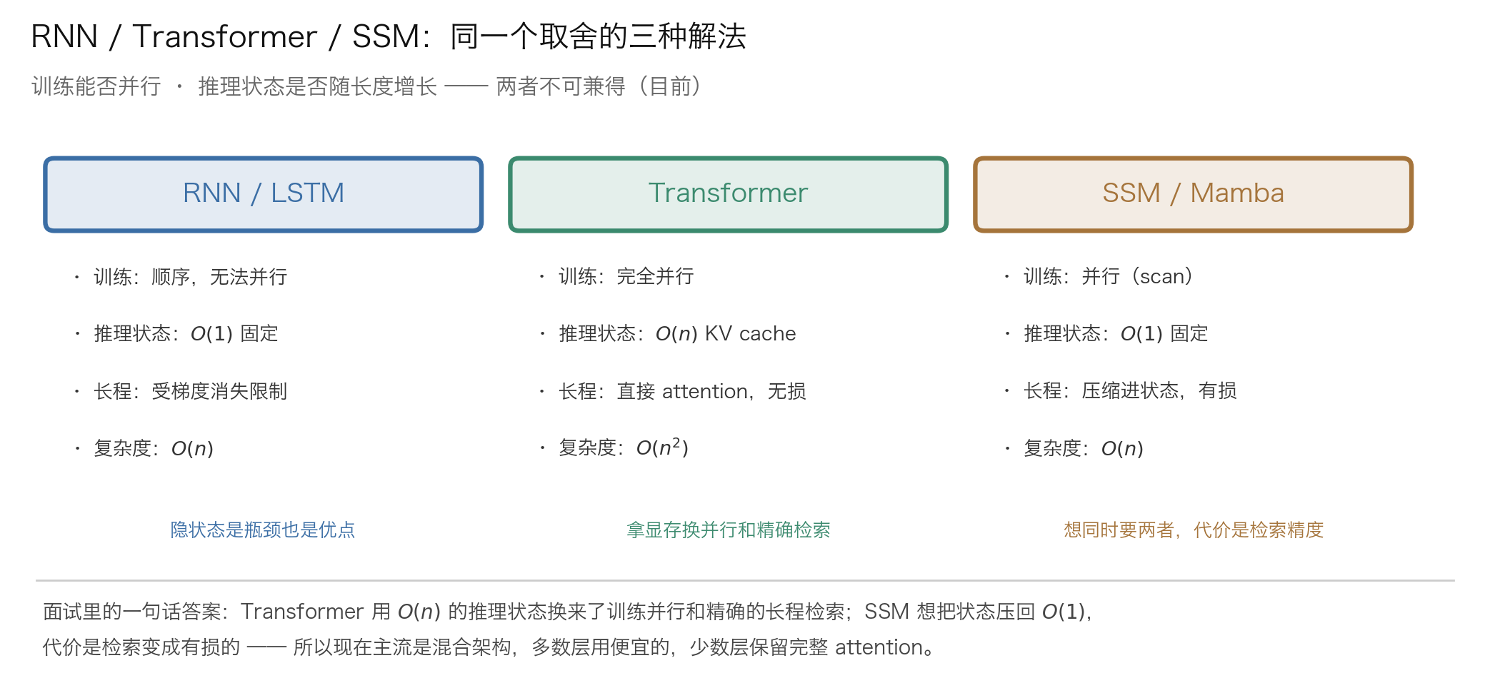
The core trade-off is state size.
| State | Training | Inference per token | Weakness | |
|---|---|---|---|---|
| Attention | \(O(n)\) (KV cache) | Parallel | \(O(n)\) | Memory explodes at long context |
| RNN/LSTM | \(O(1)\) fixed | Sequential | \(O(1)\) | No training parallelism; forgets long range |
| SSM / Mamba | \(O(1)\) fixed | Parallel (scan) | \(O(1)\) | Weak at exact recall |
| Linear attention | \(O(1)\) fixed | Parallel | \(O(1)\) | Usually below softmax attention in quality |
What Mamba fixed. The fatal flaw of RNNs is that training cannot be parallelised. SSMs recover training parallelism with a parallel scan while keeping an \(O(1)\) inference state. Mamba’s selective mechanism makes the state transition input-dependent, so the model can decide what to remember and what to forget.
Why it has not replaced the transformer. A fixed-size state means exact recall is necessarily lossy. On a task like “find that phone number somewhere in 100k of context,” attention can just look back, while an SSM has only whatever it compressed into the state. So the mainstream answer today is hybrid architectures: mostly Mamba layers, a few attention layers, buying efficiency and exact recall at the same time.
Self-test · A2.13
Q A2.13.1 — Will state space models replace attention?
The trade-off is state size, and it is fundamental rather than an implementation detail. Attention keeps an \(O(n)\) state (the KV cache) and can therefore look back at any token exactly. SSMs keep an \(O(1)\) state, so recall is necessarily lossy — anything not compressed into the state is gone.
That predicts exactly what is observed: SSMs are competitive on language modelling loss and much cheaper at long context, but weaker on tasks that need precise retrieval from far back, which is what most agentic and long-document workloads need.
So the answer is probably not replacement but hybrids — mostly SSM layers for cheap sequence mixing, a few attention layers for exact recall. Several recent models ship this.
Follow-ups
- What did Mamba fix about RNNs? → Training parallelism, via a parallel scan, while keeping the \(O(1)\) inference state. The selective mechanism makes the state transition input-dependent, so the model chooses what to keep.
- Why is linear attention weaker? → Removing the softmax makes the attention matrix low-rank, so it cannot represent sharp, selective attention patterns.
Concepts still to add: the implementation details of cross-attention; ALiBi and relative position biases; nGPT and other normalisation variants; diffusion language models; architecture search and the history behind “why are these hyperparameters these values.”
A3 · Common models
★ An entirely new section. Its value is not the catalogue but that it forces you to connect architectural choices to constraints: why does Llama 3 use GQA while DeepSeek uses MLA? Why was DeepSeek-V3 willing to drop the auxiliary loss?
This section is also the ammunition for the most frequent question of all: “what have you been following lately?” When it comes, you need to be able to say what different choice a model made, and why — not recite parameter counts.
A3.1 One comparison table
| Llama 3 70B | DeepSeek-V3 | Qwen3 | Mixtral 8×7B | |
|---|---|---|---|---|
| Type | Dense | MoE | Dense + MoE, two lines | MoE |
| Parameters | 70B | 671B total / 37B activated | 0.6B–235B | 47B total / 13B activated |
| Attention | GQA (8 KV heads) | MLA | GQA | GQA |
| FFN | SwiGLU | DeepSeekMoE + shared experts | SwiGLU / MoE | top-2 of 8 experts |
| Norm | RMSNorm, pre-LN | RMSNorm, pre-LN | RMSNorm + QK-norm | RMSNorm |
| Position | RoPE | RoPE (decoupled) | RoPE | RoPE |
| Vocabulary | 128k | 129k | 151k | 32k |
| Training tokens | ~15T | 14.8T | ~36T | — |
| Precision | bf16 | FP8 mixed precision | bf16 | bf16 |
| The one thing worth remembering | Even the 8B saw 15T, far past Chinchilla | Aux-loss-free load balancing + MTP | Hybrid thinking mode | Brought MoE into the mainstream |
How to use this table. Do not memorise it. Pick three columns and be able to say, for each, what different choice it made and which constraint that solved. What the interviewer wants is that you can map choices to constraints, not that you can recall.
Self-test · A3.1
Q A3.1.1 — Pick one recent model and tell me what is interesting about it.
A good answer picks one design decision and traces it to a constraint. For example, DeepSeek-V3:
“The interesting thing is that they attacked three different costs at once. MLA compresses the KV cache into a low-rank latent — and unusually their ablations show it beating MHA on quality, not just matching it, so it is not a trade-off. They dropped the MoE auxiliary loss in favour of a bias term adjusted during training, because an auxiliary loss adds a gradient that fights the language-modeling objective. And they trained in FP8 with per-tile scaling, which is the first large-scale demonstration that FP8 pretraining is stable.”
That is three specific choices, each tied to a constraint, in 30 seconds.
Follow-ups
- Why is per-tile FP8 scaling needed? → FP8’s dynamic range is too narrow for one global scale to cover a whole tensor, so outliers either saturate or crush the resolution of normal values.
Traps
- Reciting the spec sheet without naming a single constraint any design choice was solving. The table is an index, not an answer.
A3.2 Llama 3: throwing Chinchilla out
The key decision: the 8B model was trained on ~15T tokens, which is 90× the Chinchilla-optimal point (roughly 160B tokens).
Why. Chinchilla optimises training compute. If a model is going to serve hundreds of millions of requests and inference dominates total cost, then training a smaller model for longer is the rational move — it is cheaper on every request forever, while the extra training is paid once.
Other things worth saying:
- GQA across the whole family, including the 8B. The KV cache is the precondition for long context being viable.
- A 128k vocabulary (up sharply from Llama 2’s 32k), mostly for multilingual token efficiency.
- The 405B used bf16 and not FP8 — an explicit choice to stay conservative, putting stability ahead of efficiency.
Self-test · A3.2
Q A3.2.1 — Llama 3 8B was trained on ~15T tokens. Is that a mistake?
No — it is a deliberate re-framing of what is being optimised. Chinchilla gives the compute-optimal point for training. Once you account for inference over the model’s lifetime, the optimum moves strongly toward smaller-and-longer: a smaller model is cheaper on every single request, forever, while the extra training is paid once.
The regime is sometimes called “inference-optimal.” The limit is data: at some point you run out of high-quality tokens and start repeating, and returns collapse after roughly 4 epochs.
Follow-ups
- So is Chinchilla wrong? → No, it answers a different question correctly. Always ask “optimal for training cost or for total lifetime cost?”
Traps
- Saying Llama 3 “violates the scaling laws.” It does not — it optimises a different objective: total lifetime cost rather than training cost.
A3.3 DeepSeek-V3 / R1: three choices worth learning from
1. MLA (Multi-head Latent Attention). Compress K/V into a low-rank latent (512 dimensions) and cache that, plus a 64-dimensional decoupled RoPE key (RoPE is position-dependent, so it cannot be absorbed into the compression). Compared under the same 70B configuration as the table in A2.5 (\(L=80\)), that is about 90 KiB per token, more than an order of magnitude below MHA’s 2,560 KiB. DeepSeek-V3 itself has 61 layers, so its real number is smaller still. And their ablations show MLA modelling better than MHA — GQA is slightly worse than MHA; MLA is not.
2. Batch-level load balancing without an auxiliary loss. Conventional MoE uses an auxiliary loss to force the router toward balance, but that loss competes for gradient with the language-modeling objective. DeepSeek instead gives each expert a bias term adjusted dynamically during training: lower it when the expert is overloaded, raise it when underloaded. Balance is achieved by shifting the routing decision rather than by adding an adversarial gradient. To be precise this is batch-level — they still keep a sequence-level balance loss at \(\alpha=10^{-4}\).
3. FP8 mixed-precision training. Per-tile / per-block scaling instead of a single global scale.
R1: RLVR makes long reasoning emerge. R1-Zero runs verifiable-reward RL directly on the base model with no SFT cold start, and long-chain reasoning grew on its own — including backtracking behaviour like “wait, let me check that again.” That is strong evidence that reasoning can be elicited by reward rather than having to be demonstrated. The released R1 does add a cold-start SFT, mainly for readability.
Self-test · A3.3
Q A3.3.1 — Why does MLA beat GQA, when both reduce the KV cache?
They compress along different axes. GQA shares K/V heads across query groups — it throws away head diversity, and the ablations show a small quality cost versus MHA.
MLA projects K/V into a low-rank latent and reconstructs them per head. Each head still gets its own K/V, they are just derived from a shared compressed representation. Because the projection is learned, it can keep the directions that matter — and it acts as a mild regulariser, which is the usual explanation for why it came out slightly better than MHA in their ablations.
The cost is complexity: you need the decoupled RoPE key, and the implementation is markedly harder than repeat_interleave.
Follow-ups
- Why can’t RoPE be absorbed into the compression? → RoPE applies a position-dependent rotation. The compressed latent is cached once and reused across positions, so a position-dependent transform cannot be folded into it. Hence a small separate key that carries position.
Q A3.3.2 — What is wrong with the MoE auxiliary loss?
It is a second objective competing with the first. The gradient from the balance loss pushes the router toward uniformity regardless of whether uniform routing is good for the language-modeling loss, so you trade quality for balance and have to tune the coefficient to manage that trade.
DeepSeek’s alternative takes batch-level balancing out of the gradient: a per-expert bias, adjusted between steps from observed load, shifts the routing decision while contributing no gradient of its own. Balance becomes a control problem rather than an optimisation term.
Be accurate about the scope if pushed — they did not remove auxiliary losses altogether. A sequence-level balance loss with \(\alpha = 10^{-4}\) remains, guarding against extreme imbalance inside a single sequence.
Follow-ups
- What are shared experts? → Experts every token visits, alongside the routed ones. Common knowledge lives there instead of being replicated across every specialist, so the routed experts can actually specialise.
Traps
- Saying MLA “is just a kind of GQA.” GQA shares K/V heads; MLA compresses to a low-rank latent and reconstructs. Different axes of compression.
- Saying the aux loss was dropped to save compute. It was dropped to remove a gradient that fights the language-modeling objective.
A3.4 Qwen3 and hybrid thinking
Hybrid thinking mode. One model supports both a “thinking” and a “non-thinking” mode, switched by the user or by the template. Thinking mode emits a long CoT; non-thinking mode answers directly.
Why this is a good design. Reasoning is expensive and most requests do not need it. Handing the decision to the caller avoids the “either everything is slow or everything is dumb” dilemma. It also solves a product problem along the way: users can see what they are paying for.
Also: about 36T training tokens (more than Llama 3); two product lines, dense and MoE; and QK-norm (RMSNorm on Q and K before the dot product) to keep attention logits stable at scale.
Self-test · A3.4
Q A3.4.1 — What problem does QK-normalisation solve?
The \(1/\sqrt{d_k}\) scaling argument assumes q and k have unit-variance components. That holds at initialisation and stops holding as weights drift — at large scale attention logits can grow until the softmax saturates and training destabilises.
QK-norm applies RMSNorm to Q and K before the dot product, which bounds their magnitude directly rather than relying on an initialisation-time argument. It costs two extra normalisations per layer and buys stability at scale.
Follow-ups
- Is this related to attention entropy collapse? → Yes. Saturated softmax means near-zero attention entropy, which is a documented instability mode in large training runs.
Traps
- Conflating QK-norm with the pre-LN norm. The former acts on Q/K and specifically targets logit growth; the latter acts on the sublayer input.
A3.5 Mixtral and the mainstreaming of MoE
Mixtral 8×7B is the model that brought MoE into the open-source mainstream: 8 experts, top-2 per token, 47B total parameters but only about 13B activated per token.
The accounting it taught everyone (which matters more than the model itself):
- Memory is counted from total parameters (all experts must be resident): 47B
- Compute is counted from activated parameters (only 2 experts participate): 13B
- So it delivers quality near the 47B tier, speed near the 13B tier, and memory demands at the 47B tier
That “memory expensive, compute cheap” profile determines where MoE fits: serving that is throughput-first with memory to spare, and not edge deployment.
Self-test · A3.5
Q A3.5.1 — For a fixed serving budget, would you pick a 47B MoE or a 13B dense model?
Ask what the budget is denominated in.
Memory-bound (a single card, or long context where KV cache dominates): the dense 13B, because the MoE needs all 47B of weights resident regardless of how few are active.
Throughput-bound with memory to spare: the MoE, because you get near-47B quality at near-13B compute per token.
There is also a serving-complexity cost: expert parallelism means all-to-all on every MoE layer, and load is data-dependent, so batching and balancing are harder.
Follow-ups
- How do you compute training FLOPs for a MoE? → \(6ND\) with \(N\) = activated parameters. Using total parameters overestimates by the sparsity factor.
Concepts still to add: GPT-OSS and open-weight models; Gemma’s sliding-window interleaving; Kimi/Moonshot’s practical experience with the Muon optimizer; what can be inferred about the architecture of closed models; how to read a model card and a system card.
Traps
- Computing MoE training FLOPs from total parameters. Use activated parameters.
A4 · Pretraining
★ An entirely new section. Pretraining used to be scattered across three places (parallelism in A5, data in A9, scaling laws in A11), but no section covered pretraining itself — the objective, the end-to-end procedure, how the hyperparameters get set, and what the training dynamics should look like.
A4.1 The training objective: why next-token prediction
The objective is simply the negative log-likelihood of the sequence:
\[\mathcal L(\theta)=-\sum_{t=1}^{T}\log p_\theta(x_t\mid x_{<t})\]Because the target distribution is one-hot, \(H(p)=0\), so cross-entropy is the KL divergence — minimising CE is exactly minimising the KL to the data distribution (see A1.9).
Why it is so strong. Three reasons, and give more than one in an interview:
- Maximum signal density. Every position is a supervised prediction. MLM masks only ~15% of tokens, so for the same data you get roughly 6× less signal.
- It is a “compression is understanding” objective. To predict the next word well you are forced to learn syntax, facts, reasoning, even the speaker’s intent — because all of those are ways to lower perplexity.
- Training and usage are the same operation. No task head is needed; prompting turns almost every task into generation.
A variant: multi-token prediction (MTP). Each position additionally predicts several future tokens. Keep the two designs apart: Gloeckle et al. (2024) use 4 independent parallel heads; DeepSeek-V3 uses a sequential module of depth \(D=1\), so it predicts only 1 extra token, and it shares the embedding and output head with the main model while preserving the causal chain. Both densify the signal, and both hand you a draft model for free for speculative decoding.
A limitation worth raising unprompted. Next-token prediction is behavioural cloning: it learns what human-written text looks like, not what is correct. Recovering from its own errors and expressing uncertainty are both outside this objective — which is exactly why post-training exists.
Self-test · A4.1
Q A4.1.1 — Why did masked language modelling lose to next-token prediction?
Signal density is the main argument: MLM supervises ~15% of positions, next-token supervises 100%. At fixed compute you get roughly 6× more gradient signal per token of data.
Two more: MLM needs a task-specific head for downstream use, while a decoder-only LM does everything through generation; and MLM’s train/test mismatch (it never generates during training) makes it unnatural for the generative tasks that turned out to matter.
BERT-style models are still the right choice for embedding and retrieval, where you encode a fixed input and want every token to see the whole sequence.
Follow-ups
- Could you train with both objectives? → People have (UL2, prefix-LM). The gains are modest and the complexity is real, so the field consolidated on decoder-only.
Traps
- Saying MLM is “worse.” It is still the better objective for embedding and retrieval.
Q A4.1.2 — What does multi-token prediction buy, and what does it cost?
Denser training signal (each position supervises several future tokens), a better internal representation of “where this is going,” and a free draft model for speculative decoding.
Cost depends on the variant. Parallel heads (Gloeckle et al.) add real parameters and compute. DeepSeek-V3’s sequential module shares the embedding and output head, so the marginal cost is one transformer block plus a projection per depth — and they use depth 1. Either way the auxiliary losses need weighting, and the extra prediction machinery is usually discarded after pretraining unless you keep it for speculation.
A4.2 The order of operations for training a model from scratch
A checklist worth committing to memory. When an interview asks “how would you train a model from scratch,” go in this order.
- Fix the budget. How many GPUs, how many days → total FLOPs \(C\). Everything downstream follows from this.
- Fix the model and data sizes. Back out \(N\) and \(D\) from \(C\) and Chinchilla (or from your own inference-cost reasoning).
- Train the tokenizer. Train BPE on the target data distribution and fix the vocabulary size (larger for multilingual). Once this is locked in, it is extremely hard to change.
- Build the data pipeline. Collect → extract → filter → deduplicate → decontaminate → mix (see A9).
- Fix the architecture. Depth-to-width ratio, attention variant (GQA/MLA), FFN type, positional encoding, norm placement.
- Set hyperparameters with a small proxy model. muP makes the optimal LR width-invariant, so you can sweep on a small model.
- Do a short validation run. A few hundred steps: check that loss falls, check MFU, memory, and that checkpoints save and load.
- Launch, and watch the dashboard. Loss, gradient norm (pre-clip), MFU, agreement across ranks.
- Midtrain. Long-context extension plus a high-quality data anneal (see A9.3).
- Evaluate and decide. Held-out loss plus target benchmarks, to judge whether to continue, roll back, or move to post-training.
Step 7 is the one people skip. A few hundred steps catch 90% of configuration errors at one ten-thousandth of the cost of the whole run. Launching straight into the big run and then finding a data-sampler bug at step 40k is something that genuinely happens (see A5.5).
Self-test · A4.2
Q A4.2.1 — You have 512 H100s for one month. Walk me through planning the run.
Compute budget first. \(512 \times 9.89\times10^{14} \times 0.40 \times 30\times86400 \approx 5.2\times10^{23}\) FLOPs at 40% MFU.
Then size the model. With \(C = 6ND\) and Chinchilla’s \(D \approx 20N\): \(C = 120N^2 \Rightarrow N = \sqrt{C/120} \approx 6.6\times10^{10}\) — about a 66B model on 1.3T tokens.
Then reality-check that against serving. If this model will be served heavily, Chinchilla-optimal is the wrong target — train something smaller for longer. A 20B model on 4T tokens uses the same compute and is 3× cheaper to serve.
Then the rest of the checklist: tokenizer, data pipeline, architecture, small-proxy hyperparameter sweep, short validation run, launch.
Follow-ups
- What would make you deviate from Chinchilla? → Inference cost dominance, data scarcity in the target domain, or a fixed memory budget on the serving side.
- What is the first thing you check after launch? → That loss is falling and MFU is where the short run said it would be. If MFU is half of what you measured, stop and find out why before burning a month.
Traps
- Skipping the step-7 short validation run and going straight to the full run. A few hundred steps catch nine configuration errors out of ten, at one ten-thousandth of the cost.
A4.3 Choosing the architecture and hyperparameters
Shape (wide vs deep). For a parameter budget \(N \approx 12LD^2\) there are many \((L, D)\) combinations to choose from. What experience says:
- Too deep and narrow → more pipeline stages and a bigger bubble, plus skinny per-layer matrices and low MFU.
- Too wide and shallow → not enough expressive depth, and TP communication grows with \(D\).
- In practice \(D/L\) lands around 100–150 (Llama-3-70B: \(8192/80 = 102\)).
Everything else you have to pin down:
| Choice | Modern default | Reason |
|---|---|---|
| Attention | GQA (\(K=8\)) or MLA | The KV cache is the long-context bottleneck |
| FFN | SwiGLU, \(F=\tfrac83 D\) | Empirically better at equal parameters |
| Norm | RMSNorm, pre-LN | Fewer reductions; removes the architectural need for warmup (you still warm up, see A1.6) |
| Position | RoPE | Relative, and extrapolates when scaled |
| Vocabulary | 32k–256k | Larger for multilingual; drives \(2VD\) |
| Initialisation | \(\mathcal N(0, 0.02)\), residual layers scaled by \(1/\sqrt{2L}\) | Controls residual-stream growth |
Hyperparameters. Batch size is counted in tokens (millions) and grows with scale. LR falls with scale — which is exactly what muP is for. Warmup is 1–2% of total steps. Weight decay 0.1. \(\beta_2=0.95\) rather than 0.999.
Why residual layers are initialised with a \(1/\sqrt{2L}\) scaling. Under pre-LN the variance of the residual stream accumulates with depth. If every layer’s output is \(O(1)\), after \(L\) layers the stream has magnitude \(O(\sqrt L)\) and the later layers matter relatively less and less. Scaling the initialisation by depth keeps each layer’s relative contribution constant.
Self-test · A4.3
Q A4.3.1 — How do you choose the width-to-depth ratio?
There is a broad plateau, so it is not a delicate choice — but the failure modes at the ends are real. Too deep and narrow: more pipeline stages (bigger bubble), skinny matmuls (low MFU), and harder optimisation. Too wide and shallow: less compositional depth, and TP communication grows with \(D\).
Practical anchors: \(D/L \approx 100\)–\(150\). Llama-3-70B is \(8192/80 = 102\).
The systems consideration usually decides it: depth costs you pipeline bubble, width costs you tensor-parallel bandwidth. Pick the one your interconnect tolerates.
Follow-ups
- Does the optimal ratio change with scale? → Slowly — larger models get somewhat wider relative to depth. The scaling-law papers fit this explicitly.
Traps
- Saying “deeper is always better.” Depth buys you pipeline bubble and skinnier matrices; both ends cost something.
Q A4.3.2 — Why is the peak learning rate smaller for larger models?
Under standard parameterisation the scale of the update relative to the weight grows with width, so the stable LR shrinks — empirically roughly \(\propto 1/\sqrt{D}\) or fitted as \(\text{LR}(C)=\beta C^{-\alpha}\).
muP fixes this by rescaling initialisation and per-layer learning rates so the relative update magnitude is width-invariant. Then the optimal LR transfers from a small proxy, which is the only practical way to tune a run you can afford once.
A4.4 Training dynamics: what the curves should look like
A normal loss curve is close to a straight line in log-log (a power law), made up of:
- a steep drop over the first few hundred steps (learning the token frequency distribution — the unigram baseline);
- then a long, smooth power-law stretch;
- plus an extra accelerated drop during the LR decay phase.
Four lines to watch at once — loss alone is not enough:
| Metric | Normal | What abnormal means |
|---|---|---|
| Loss | Smooth power law | Spikes → see A5.5 |
| Gradient norm (pre-clip) | Steady, occasional small peaks | Rising persistently → instability is brewing |
| MFU | Constant | Falling → communication or data-pipeline problem |
| Loss agreement across ranks | Consistent | One rank drifting → hardware problem |
The gradient norm is the earliest warning, and it is only useful if you log the pre-clip value. Plenty of people log only the post-clip norm, which is flat by construction and shows nothing.
When to stop. If held-out loss is still falling, usually keep going — pretraining rarely truly saturates, and stopping is normally a budget decision rather than a returns decision. The real stop signals are: held-out loss flat while training loss keeps falling (overfitting, meaning the data is repeating), or the benchmarks for the capability you care about no longer moving.
Self-test · A4.4
Q A4.4.1 — Your loss curve has a long flat plateau at the start before dropping. What is happening?
Almost always the learning rate is too low, or warmup is too long. The model is stuck near the unigram solution — it has learned token frequencies and nothing else.
Diagnostic: check whether the loss value matches the entropy of the unigram distribution over your corpus. If it does, the model is producing a frequency-matched distribution and no context is being used. Then print the actual LR after warmup (not the config value) — an off-by-one in the scheduler is a common cause.
Follow-ups
- What if loss drops fast then plateaus high? → Possible label/shift bug, or a data pipeline returning something degenerate. Overfit ten examples to isolate.
Traps
- Watching loss only. Gradient norm, MFU and cross-rank agreement have to be read together — and the gradient norm has to be the pre-clip one.
Q A4.4.2 — Why log the gradient norm before clipping?
Because after clipping the series is flat by construction — you have destroyed the signal you wanted to monitor. The pre-clip norm rising over time is the earliest indication that instability is developing, often hundreds of steps before it shows in the loss.
It also tells you whether clipping is active. If most steps are being clipped, the clip threshold is doing the work of a learning rate, which means your LR is too high.
A4.5 Checkpointing and fault tolerance
Why this is a first-class pretraining problem. Over a 90-day run hardware failures are certain. GPUs drop out, nodes die, NCCL times out. With no fault-tolerance design, a single failure costs you all the compute since the last checkpoint.
What to save. Model weights, optimizer states (the bulk of it, \(8P\)), the LR scheduler state, and the data sampler position.
That last item is the easiest to forget and the most damaging to forget. If the data sampler does not restore its position on resume, the model re-reads tokens it has already seen. Bekman’s warning: you may only find out afterwards that you “turned 300B tokens that were each meant to be seen once into the same 50B tokens trained 6 times.” That is not a spike; that is a run silently invalidated.
How to set the frequency. With a mean time between failures MTBF and a checkpoint interval \(T_c\), the expected loss per failure is about \(T_c/2\) of compute. Rule of thumb: \(T_c\) of 15–30 minutes, far below MTBF. But the write itself must not slow training down — use asynchronous writes and sharded checkpoints (each rank writes only its own shard).
Self-test · A4.5
Q A4.5.1 — Design the checkpointing strategy for a 90-day run on 2048 GPUs.
What to save: weights, optimizer states, scheduler state, RNG states, and the data sampler position. Missing the last one silently invalidates the run.
Frequency: if MTBF is ~4 hours at this scale, checkpoint every 15–30 minutes; expected loss on a failure is then under 15 minutes of compute.
Make the write cheap: sharded (each rank writes its own shard, no gather), asynchronous (copy to host memory, then flush in the background so training continues), and keep a rolling window of the last \(k\) plus periodic permanent ones — you may need to roll back further than one checkpoint if a divergence is discovered late.
Also plan the restart: automatic detection (a watchdog on step progress, not just process liveness — a hung NCCL collective keeps the process alive), and a spare-node pool so restart does not wait on provisioning.
Follow-ups
- How do you verify a checkpoint is loadable? → Restore it in a separate job and check that loss on a fixed batch matches. A checkpoint you have never restored is not a checkpoint.
- Why keep several permanent ones? → Because a slow-developing divergence may only be visible thousands of steps later, and you need somewhere clean to go back to.
Traps
- Checkpointing only weights and optimizer states, and forgetting the data sampler position.
A4.6 Evaluation during pretraining
The primary metric is held-out loss, not benchmarks. The reasons: it is smooth, comparable, low-variance, and computable at every step, whereas benchmarks are discrete, noisy, and can be contaminated.
But loss alone is not enough. Pair it with:
- Per-domain held-out loss (one each for code, maths, multilingual) — an aggregate loss hides one domain gaining while another loses.
- A few cheap benchmarks, run periodically, read as trends rather than absolute values.
- Qualitative sampling. Read a few dozen generations regularly. This is the easiest step to skip and the easiest way to catch problems loss cannot show you (repetition loops, broken formatting).
Do not run large benchmarks frequently during pretraining. They are slow, they are noisy, and they tempt you into making decisions against noise. A small suite once a day plus a full evaluation at milestones is enough.
Self-test · A4.6
Q A4.6.1 — Why is held-out loss a better training-time metric than MMLU?
Loss is continuous, low-variance, computable every step, and comparable across checkpoints of the same tokenizer. Benchmark accuracy is thresholded (exact match), which makes it discontinuous and noisy — a model can improve substantially with no benchmark movement, and can move on a benchmark from run-to-run noise alone.
The catch: loss is not comparable across tokenizers, and after post-training it stops tracking usefulness at all. Use bits-per-byte if you must compare across tokenizers.
Follow-ups
- When would you look at benchmarks during pretraining? → At milestones, to decide whether to continue, change the data mix, or stop. Not for step-to-step decisions.
Concepts still to add: continued pretraining and domain adaptation; numerical mismatch between training and inference; model merging (model soup); how to read a public training logbook.
Traps
- Running large benchmarks frequently during pretraining. Slow, noisy, and it tempts you into deciding against noise.
A5 · Training infrastructure
Parallelism, precision, stability, MFU — these apply to both pretraining and post-training, so they get their own section.
The dividing line for this section: name which memory term you ran out of first, then say which parallelism you reach for. The other order is just reciting vocabulary.
A5.1 Where the memory goes
Write the memory equation before you talk strategy. The order itself is the signal.
\[\text{memory} = \underbrace{P}_{\text{params}} + \underbrace{P}_{\text{grads}} + \underbrace{2P\text{–}4P}_{\text{optimizer}} + \underbrace{\text{activations}}_{\propto BS}\]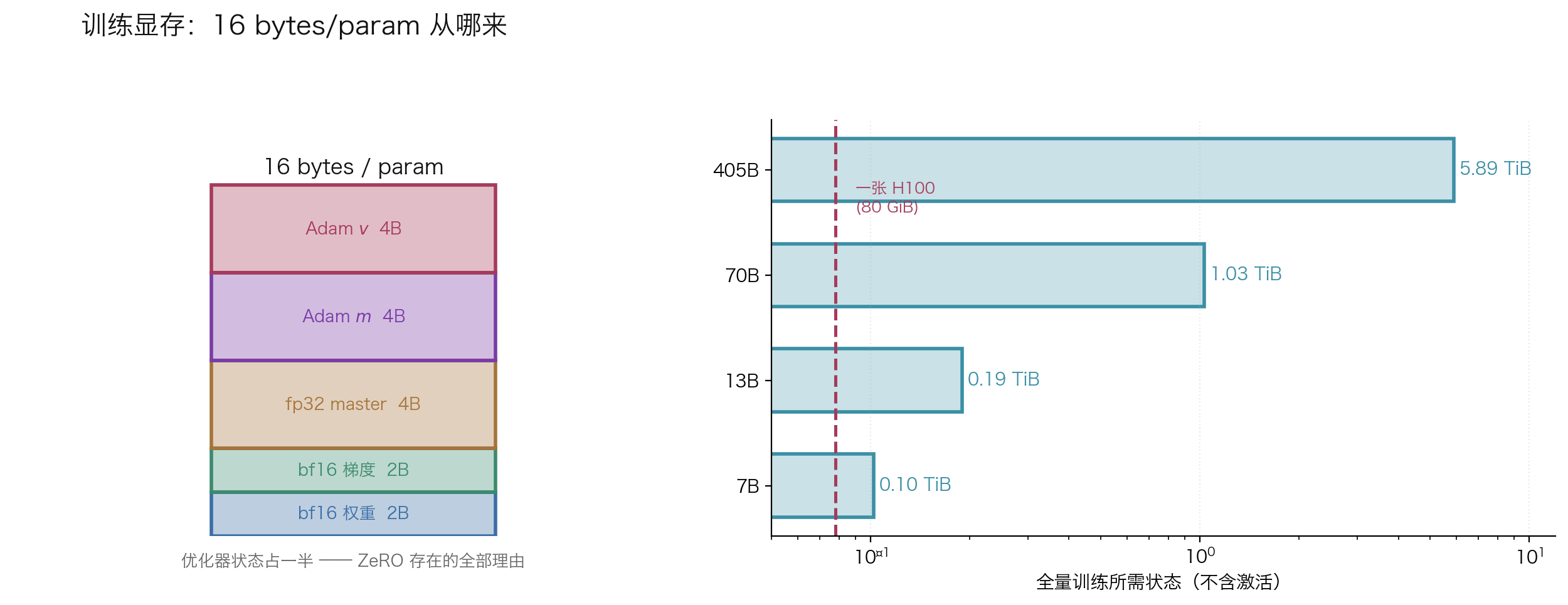
The standard mixed-precision + AdamW accounting (bytes per parameter):
| Item | Precision | Bytes/param |
|---|---|---|
| bf16 weights | bf16 | 2 |
| bf16 gradients | bf16 | 2 |
| fp32 master weights | fp32 | 4 |
| Adam first moment | fp32 | 4 |
| Adam second moment | fp32 | 4 |
| Total | 16 |
So a 70B model is 1,120 GB in state alone, before a single activation. This is why training a large model on one card was never on the table.
Activations are the other half of the story, and they grow with \(B\times S\), which makes them the dominant term in long-context training. Gradient checkpointing buys most of that memory back for about 30% extra compute.
Self-test · A5.1
Q A5.1.1 — Explain gradient checkpointing. What does it cost and when is it not worth it?
Activations have to be kept from the forward pass because the backward needs them. Checkpointing keeps only a subset — typically one tensor per layer boundary — and recomputes the rest during backward from the nearest saved point.
The standard trade is roughly 30% more compute for most of the activation memory. The clean way to state it: with \(L\) layers, checkpointing every \(\sqrt{L}\) layers gives \(O(\sqrt L)\) memory instead of \(O(L)\) at the cost of one extra forward pass.
When it is not worth it: when activations were not your binding constraint (you are limited by optimizer state, so shard that instead), or when you are already compute-bound and latency matters more than fitting a bigger batch.
One reporting subtlety worth mentioning: recomputation is not in the \(6N\) numerator, so turning on checkpointing lowers MFU even when it raises tokens/second. Compare HFU if you want to see the hardware picture (see A5.4).
Q A5.1.2 — Why is it 16 bytes per parameter and not 6?
Because the optimizer dominates. Weights and gradients in bf16 are 2 bytes each; the fp32 master copy is 4; Adam’s two moment estimates are 4 each in fp32. Twelve of the sixteen bytes are optimizer and master state, which is exactly why ZeRO shards those first — stage 1 alone removes the largest term.
The figure is sometimes quoted as 18. That depends on whether gradients are accumulated in fp32 and whether a transient bf16 copy is counted, so state the standard recipe and note it is framework-dependent.
Follow-ups
- What does SGD with momentum cost? → 4 bytes fewer per parameter (one moment instead of two). It is not used for LLMs because Adam’s per-parameter scaling matters a lot for transformers.
A5.2 Parallelism strategies: what each one shards
| Strategy | What it shards | Communication | Where it breaks |
|---|---|---|---|
| DDP | Nothing | Gradient all-reduce | Every device must hold the full state |
| ZeRO-1 | Optimizer state | reduce-scatter + all-gather | — |
| ZeRO-2 | + gradients | Same | — |
| ZeRO-3 / FSDP | + parameters | Per-layer gather | Communication volume grows |
| Tensor (TP) | Parameters and activations inside a layer | Two all-reduces within every layer | Needs NVLink; do not cross nodes |
| Pipeline (PP) | Groups of layers | Point-to-point at the boundaries | Bubble \(\approx (p-1)/(m+p-1)\) |
| Context / Ring | The sequence | Ring exchange of K/V | Only fixes activations |
| Expert (EP) | Experts | all-to-all | Load imbalance |
| Recompute | — | None | ~30% compute for activation memory |
3D parallelism = DP × TP × PP. The standard layout: TP innermost, inside a node (it is the bandwidth hog), PP across nodes (lowest volume), DP outermost.
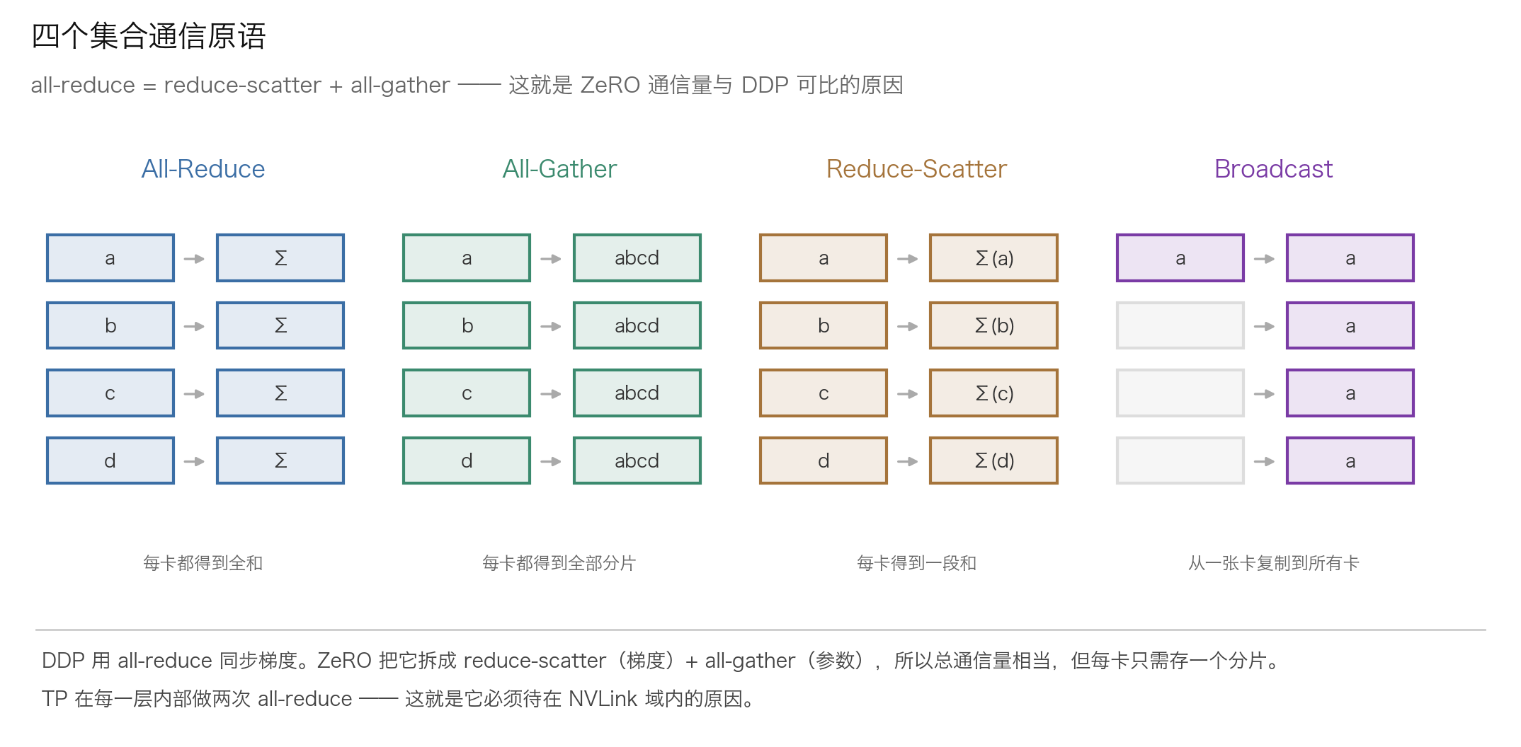
The collective primitives: all-reduce (sum, everyone gets the result), all-gather (concatenate, everyone gets everything), reduce-scatter (sum, everyone gets one slice). Note that all-reduce = reduce-scatter + all-gather, which is exactly why ZeRO’s communication cost comes out comparable to DDP’s.
Self-test · A5.2
Q A5.2.1 — You are out of memory training a large model. Walk through the options.
Start from which term is too big, not from the list of strategies.
If optimizer state dominates, ZeRO-1 then ZeRO-2 — they shard the twelve heaviest of the sixteen bytes with communication volume comparable to DDP, so they are nearly free.
If parameters do not fit, ZeRO-3/FSDP or tensor parallelism. TP within a node only: it does two all-reduces per layer, and inter-node bandwidth is an order of magnitude below NVLink, so crossing nodes eats the benefit immediately.
If activations dominate — which is the usual case at long context — gradient checkpointing first (about 30% more compute for most of the memory), then context/sequence parallelism.
If the model is too deep for any of that, pipeline parallelism across nodes, accepting the \((p-1)/(m+p-1)\) bubble and using enough micro-batches to shrink it.
Follow-ups
- How do you shrink the pipeline bubble? → More micro-batches, interleaved 1F1B, or zero-bubble schedules that split the backward into input-gradient and weight-gradient halves.
- Why is ZeRO’s comm cost comparable to DDP’s? → Because all-reduce is literally reduce-scatter followed by all-gather, which is what ZeRO-1/2 do anyway.
Traps
- Naming a strategy before naming the problem. Say which memory term you ran out of first — that is what the interviewer is waiting for.
A5.3 Mixed precision
The recipe. fp32 master weights; forward and backward in low precision; the optimizer update applies to the master copy.
Why the master copy. Updates are usually orders of magnitude smaller than the weights. bf16 has 7 mantissa bits, a relative precision of about \(2^{-8}\approx 0.4\%\). Once \(|\Delta w|/|w| < 0.4\%\), the addition rounds straight back to \(w\) — the model quietly stops learning while the loss curve still looks reasonable.
bf16 vs fp16. Same width, different split: fp16 is 5 exponent + 10 mantissa, bf16 is 8 + 7. Eight exponent bits give bf16 the same dynamic range as fp32 — attention logits do not overflow, and you need none of the loss-scaling machinery. The price is mantissa precision, and training turns out not to care.
fp16 forces dynamic loss scaling: scale the loss up before the backward so small gradients land in representable range, scale it back down before the optimizer step, and back off on inf. That machinery is a classic source of silent stalls.
What has to stay in fp32: reductions. Softmax denominators, layer-norm statistics, loss accumulation, gradient all-reduce.
Self-test · A5.3
Q A5.3.1 — Why did bf16 replace fp16?
Dynamic range. Both are 16 bits, but fp16 splits them 5 exponent + 10 mantissa while bf16 splits them 8 + 7. Eight exponent bits gives bf16 the same range as fp32, so attention logits and gradients do not overflow and you need no loss-scaling machinery at all.
The trade is mantissa precision, and empirically training does not care much — which is a nice example of choosing the axis that matters rather than the bigger number.
Follow-ups
- FP8? → DeepSeek-V3 trained at scale in FP8 using per-tile and per-block scaling, because FP8’s range is too narrow for one global scale to cover a tensor. The gains are real; the numerical engineering is genuinely hard.
Traps
- Saying bf16 is “more precise.” It is less precise; it wins on dynamic range.
A5.4 MFU
\[\text{MFU} = \frac{6N\cdot(\text{tokens/s})}{\text{GPUs}\times\text{peak FLOP/s}}\]The numerator is the FLOPs the model requires (\(6N\) per token) — no recomputation, no communication. So gradient checkpointing lowers MFU even as it may raise throughput. HFU (Hardware FLOPs Utilization) counts recomputation in the numerator; MFU does not.
The healthy band for large-scale training is 35–50%. Below 30% usually means one specific thing is wrong.
Check in this order:
- Communication is not overlapped with compute. The most common cause. Is the DP all-reduce overlapping the backward? Are ZeRO-3 parameter gathers being prefetched?
- Pipeline bubble. Be careful, there are two conventions here and one follow-up question exposes it: the fraction of wall-clock spent idle is \((p-1)/(m+p-1)\), whereas the \((p-1)/m\) reported in the Megatron paper is the bubble relative to ideal compute time. At \(p=m=8\) that is 47% versus 87.5%. This section uses the wall-clock convention throughout.
- Per-device batch too small. The matmuls are too skinny to keep the hardware fed.
- The data loader is starving the GPUs. Look at the distribution of idle time, not average utilisation.
- TP is crossing a node boundary.
- Very long sequences. The \(S^2\) attention term is not in the \(6N\) numerator, so MFU reads legitimately lower at long context — a low number here is not a bug.
Self-test · A5.4
Q A5.4.1 — Your MFU is 20%. What do you check?
In order of how often it is the answer: communication not overlapped with compute (DP all-reduce not overlapping backward, or ZeRO-3 gathers not prefetched); pipeline bubble, which idles \((p-1)/(m+p-1)\) of wall-clock and is 47% on its own at \(p=m=8\); per-device batch too small for the matmuls to saturate; a data loader starving the GPUs; and tensor parallelism crossing node boundaries.
One case where 20% is correct: very long sequences. The \(S^2\) attention term is real work but is not in the \(6N\) numerator, so MFU legitimately reads low. Check HFU before chasing it.
Follow-ups
- Why not just read
nvidia-smiutilisation? → It only says a kernel is running, not that it is doing useful arithmetic. A purely memory-bound kernel shows 100%.- MoE? → Use activated parameters in the numerator, not total.
Traps
- Using the sparse peak in the denominator (H100 is 989 TFLOP/s dense; 1979 is 2:4 sparse).
A5.5 Diagnosing training instability
Do not open by lowering the learning rate. Classify the spike first — the three shapes have different causes and different fixes.
Bekman’s taxonomy: fast recovery, slow recovery, no full recovery. The usual cause: “a bad batch of data, either poorly shuffled or not cleaned properly.”
And one more detail, which is what makes this a good question:
“People suspect the batch right before the spike triggered it… but quite often the trouble has been building for many steps and only then erupts.”
The ladder, cheapest check first:
- Is it real, or a logging artifact? Does it show up in the gradient norm and the validation loss, or only in one rank’s smoothed training curve?
- Is it a resume artifact? ← The highest-value check, and almost nobody brings it up. If the run restarted and the data sampler did not restore its position, the model is re-reading tokens it has already seen. Bekman’s warning is blunt: you can find that you “trained on the same 50B tokens 6 times, instead of the 300B unique tokens you planned.” That is not spike pathology; that is a silently invalidated run.
- Hardware? One bad card is enough to poison the whole all-reduce. Check per-rank loss, ECC errors, and run a collective-communication benchmark.
- Numerics? fp16 overflow, or the loss scaler fell over. Check for inf/NaN before clipping.
- Data? Only now go and look at the batches in the window before the spike, not the one at it. Repeated tokens, a corrupted shard, a language switch.
- Optimization last. Is the LR too high for the current curvature? Are the second moments stale after a schedule change?
Match the fix to the class: fast recovery → log it and continue. Slow → lower the LR or skip that data range. No recovery → roll back to the last good checkpoint and restart with a different data order.
Self-test · A5.5
Q A5.5.1 — You are pretraining a 100B model. At step 42,000 the loss spikes. Walk me through it.
(The ladder is above.) Two things make this answer distinctive.
Classify before you act. Fast-recovering spikes are usually fine — log and continue. Slow-recovery means lower the LR or skip the data range. Non-recovery means roll back and change the data order. Reaching for the learning rate first is the common wrong move.
Check the resume path early. If the run restarted and the data sampler did not restore position, you are re-reading tokens, and that is not a spike pathology — it is a silently invalidated run. This check costs nothing and almost nobody mentions it.
And look before the spike, not at it. Instabilities usually develop over many steps, so the batch immediately preceding it is rarely the culprit.
Follow-ups
- What would you have logged in advance? → Pre-clip gradient norm (see A4.4), per-rank loss, and the data sampler’s position in every checkpoint. Most spike debugging fails for lack of these.
Traps
- Reaching for the learning rate first. The first move is to classify, and to mention the data sampler.
Concepts still to add: quantitative communication-volume analysis per ZeRO stage, NCCL tuning and topology awareness, SLURM/K8s orchestration, failure detection and auto-restart, elastic training, debugging train/inference numerical mismatch.
A6 · Post-training and RL
From SFT to RLHF to RLVR. Alisa spends 185 lines on policy gradient with the proofs written out in full; this is her deepest chapter.
The dividing line for this section: anyone can name PPO / GRPO / DPO. The signal is where the KL term sits, what shape the advantage is, and whether you can write the three derivations out.
A6.1 The post-training ladder
| Stage | Data | Can fix | Cannot fix |
|---|---|---|---|
| Pretraining | Web-scale, unlabelled | Knowledge, grammar, world model | Instruction following, format |
| Midtraining | Curated high-quality, long context, code, math | Domain capability, context length | Preferences, style |
| SFT | Demonstrations | Format, instruction following, tool syntax | Anything not demonstrated — it can only imitate |
| Reward modeling | Preference pairs | A scalar proxy for “better” | Its own misspecification |
| RL | Prompts + reward or verifier | Optimises the reward, gaming included | Knowledge the base model does not have |
| Distillation | Teacher outputs | Cost, latency | Generally cannot exceed the teacher |
A one-line frame, always available:
SFT teaches the model what a good answer looks like; RL teaches it which of its own answers are better.
This explains why RL keeps working after SFT saturates — SFT can only push toward demonstrations, while RL can rank the model’s own samples and push into territory nobody demonstrated. It also explains why RL cannot install new knowledge: it only reweights what the base model can already produce.
Self-test · A6.1
Q A6.1.1 — Lay out the stages from pretraining to a deployed model.
(The table is above.) The framing that matters: SFT teaches what a good answer looks like, RL teaches which of the model’s own answers are better. That is why RL keeps working after SFT saturates, and why RL cannot install knowledge the base model lacks — it only reweights what the policy can already produce.
Follow-ups
- Why is midtraining “the stage nobody writes down”? → It is where long-context extension, heavy code/math upweighting, and domain injection actually happen, and labs disclose almost nothing because the data mix is the moat.
- Do you need SFT before RL? → For most recipes yes — RL from base is high-variance and slow. R1-Zero showed pure RL from base can work with verifiable rewards, but the released R1 still uses a cold-start SFT stage for readability.
Traps
- Saying RL can “teach the model new knowledge.” It can only reweight capability that is already there.
A6.2 SFT: more detail than you would think
SFT looks like “just keep doing next-token prediction,” but four implementation details get asked about.
1. Loss masking. Compute the loss only on the response tokens; set the prompt labels to -100. Without the mask, the model spends capacity learning to model the prompt distribution, which is not the behaviour you want.
labels = input_ids.clone()                    # input_ids: (B, T)
for i, n in enumerate(prompt_lens):
    labels[i, :n] = -100                      # each example's own prompt length
labels[attention_mask == 0] = -100            # mask the padding too
Writing
labels[:len(prompt_ids)] = -100is the classic whiteboard slip: on a(B, T)tensor that slices the batch dimension — masking out the first few examples entirely instead of each example’s prompt. It is only correct for a single unbatched example.
2. Packing and cross-talk. Pack several short examples into one sequence for utilisation, but you must block cross-example attention (block-diagonal mask, or reset position_ids). Otherwise example B can see example A, which is a silent form of data contamination.
3. Number of epochs. SFT datasets are usually small, so 1–3 epochs. Past that it starts memorising, and both diversity and calibration degrade.
4. Quality beats quantity, by a lot. The LIMA result — a thousand carefully chosen examples beating tens of thousands of noisy ones — holds at this stage, because what you are tuning is format and behaviour, not knowledge.
Self-test · A6.2
Q A6.2.1 — Why mask the loss on prompt tokens during SFT?
Because you are training a conditional distribution \(p(\text{response}\mid\text{prompt})\), not a joint. Including prompt tokens spends capacity modelling the instruction distribution, which is not the behaviour you want and dilutes the gradient on the tokens you care about.
It matters most when prompts are long relative to responses — a 2000-token document with a 50-token answer would be 97% prompt loss, and the model would mostly be learning to predict documents.
Follow-ups
- Does it ever help to train on prompts? → Slightly, in very low-data regimes, as a regulariser. Most recipes mask.
- What breaks with packing? → Cross-contamination: without a block-diagonal mask, a packed sequence lets one example attend to another. Also remember to reset
position_ids.
A6.3 Reward models and Bradley-Terry
Train a scalar head on preference pairs:
\[\mathcal L = -\log\sigma\big(r_\theta(x,y_w) - r_\theta(x,y_l)\big)\]This is the Bradley-Terry model: it assumes the probability a human prefers \(y_w\) is \(\sigma(r_w - r_l)\).
Three things you have to be able to say:
- The reward is only determined up to an additive constant. BT constrains differences, not absolute values, so comparing raw reward numbers across runs is meaningless. Hence per-batch normalisation.
- It is trained on a narrow distribution and then queried far away from it — because the policy moves. That is a textbook Goodhart setup, and it is the entire reason the KL penalty exists.
- Wherever you can get a verifier, the verifier beats a learned reward. A unit test is a function, not a network, and cannot be gamed the same way. The causal chain from “this answer is correct” to a gradient is far shorter.
Self-test · A6.3
Q A6.3.1 — Why can’t you compare reward model scores across runs?
Bradley-Terry only constrains differences: the loss depends on \(r_w - r_l\), so adding any constant to every score leaves it unchanged. The reward is identified up to a shift, which makes the absolute scale arbitrary and run-dependent.
Consequences: normalise per batch before using rewards as advantages, do not set thresholds on raw values, and when reporting “reward went up” say what it went up relative to.
A6.4 Deriving the policy gradient
Objective. Maximise \(J(\theta) = \mathbb E_{\tau\sim\pi_\theta}[R(\tau)]\).
The derivation — the whole thing runs on one log-derivative trick, \(\nabla P = P\nabla\log P\):
\[\begin{aligned} \nabla_\theta J(\theta) &= \nabla_\theta \sum_\tau P(\tau\mid\theta)R(\tau)\\ &= \sum_\tau \nabla_\theta P(\tau\mid\theta)\,R(\tau)\\ &= \sum_\tau P(\tau\mid\theta)\,\nabla_\theta\log P(\tau\mid\theta)\,R(\tau)\\ &= \mathbb E_{\tau\sim\pi_\theta}\Big[\sum_t \nabla_\theta\log\pi_\theta(a_t\mid s_t)\,R(\tau)\Big] \end{aligned}\]Why it looks like SFT. The update is \(\nabla\log\pi_\theta(a_t\mid s_t)\) — exactly the SFT gradient — with two differences: the data \(\tau\) is sampled from the policy itself, and the gradient is weighted by \(R(\tau)\). Positive reward raises the log-probability of every token in the trajectory, negative reward lowers it, and the magnitude sets the step size.
One conceptual point worth making. The “policy gradient loss” is not a loss in the usual sense. \(L(\theta)\) does not measure how good the policy is — it is just a scalar whose .backward() happens to produce the right gradient. There is no fixed objective here, because the data distribution moves with the policy.
Self-test · A6.4
Q A6.4.1 — Derive the REINFORCE estimator and explain why it is high variance.
(The derivation is above.) The load-bearing step is the log-derivative trick, which converts a gradient of a probability into an expectation you can sample.
High variance because one scalar reward is credited to an entire trajectory. Every token gets the same weight, so on an easy prompt where the response is mostly good but contains one bad step, the bad step is reinforced too; and on a prompt where everything scores positively, all responses are reinforced including the mediocre ones. There is no per-token credit assignment in the estimator itself.
Traps
- Skipping the log-derivative trick in the derivation, or not being able to say why \(\nabla\) can move inside the sum.
A6.5 Why the baseline is unbiased
Show that the baseline term has expectation zero:
\[B = \mathbb E_{\tau}\Big[\sum_t \nabla_\theta\log\pi_\theta(a_t\mid s_t)\,b(s_t)\Big]\]Move the expectation inside the sum, then factor the joint distribution over \((s_t, a_t)\):
\[B = \sum_t \mathbb E_{s_t}\Big[\mathbb E_{a_t\mid s_t}\big[\nabla_\theta\log\pi_\theta(a_t\mid s_t)\,b(s_t)\big]\Big]\]The inner expectation:
\[\begin{aligned} \mathbb E_{a_t\mid s_t}\big[\nabla\log\pi_\theta(a_t\mid s_t)\,b(s_t)\big] &= b(s_t)\sum_{a}\pi_\theta(a\mid s_t)\nabla\log\pi_\theta(a\mid s_t)\\ &= b(s_t)\sum_{a}\nabla\pi_\theta(a\mid s_t)\\ &= b(s_t)\,\nabla\Big(\sum_a \pi_\theta(a\mid s_t)\Big) = b(s_t)\,\nabla 1 = 0 \end{aligned}\]The load-bearing step is pulling \(b(s_t)\) outside the expectation over \(a_t\) — which is legal only because \(b\) depends on the state and not the action. That single condition is the whole thing.
Why you want it. It does not change the objective, only the variance of the estimator. You want \(b(s_t)\) correlated with \(R(\tau)\) so that \(R-b\) stays small. PPO uses a learned \(V_\psi(s_t)\); GRPO uses the group mean.
Self-test · A6.5
Q A6.5.1 — Show that a state-dependent baseline does not bias the policy gradient.
(The proof is above.) The step that carries the proof is pulling \(b(s_t)\) outside the expectation over \(a_t\), which is legal only because \(b\) does not depend on the action. Then \(\sum_a \nabla\pi_\theta(a\mid s_t) = \nabla 1 = 0\).
Follow-ups
- Can the baseline depend on the action? → No — that breaks the proof and introduces bias. This is why you cannot use the sampled action’s own reward as its baseline.
- Is GRPO’s group mean action-dependent? → It is computed from other samples for the same prompt, so per-sample it is approximately independent. There is a subtle bias from including the sample itself; some implementations use a leave-one-out mean.
A6.6 PPO
The clipped surrogate. With \(r_t = \dfrac{\pi_\theta(a_t\mid s_t)}{\pi_{\theta_\text{old}}(a_t\mid s_t)}\):
\[L^{\text{CLIP}} = \mathbb E_t\Big[\min\big(r_t \hat A_t,\; \text{clip}(r_t, 1-\epsilon, 1+\epsilon)\hat A_t\big)\Big]\]What clipping buys. A soft trust region. It removes any incentive to push the probability ratio outside \(1\pm\epsilon\), so one update cannot take the policy too far — exactly what naive policy gradient lacks. The min makes it pessimistic: gains are clipped, losses are not.
GAE. The advantage interpolates between one-step TD (biased, low variance) and Monte Carlo (unbiased, high variance):
\[\delta_t = r_t + \gamma V(s_{t+1}) - V(s_t),\qquad \hat A_t = \sum_{l\ge0}(\gamma\lambda)^l\delta_{t+l}\]\(\lambda=1\) collapses to Monte Carlo, \(\lambda=0\) to one-step TD. When you implement it, assert both limits — the cheapest correctness check there is.
Four models sit in memory: the policy, a frozen reference, the reward model, and the critic.
Where the KL goes: in PPO the convention is to subtract it from the reward before computing advantages.
Self-test · A6.6
Q A6.6.1 — Write the PPO objective and explain what GAE is for.
\[L^{\text{CLIP}} = \mathbb E_t\big[\min(r_t \hat A_t,\; \text{clip}(r_t, 1-\epsilon, 1+\epsilon)\hat A_t)\big]\]with \(r_t\) the ratio of new to old policy probability. Two components and both need a reason.
The clip is a soft trust region. Plain policy gradient has nothing stopping one update from moving the policy far off the distribution the data was sampled from, which invalidates the importance weighting. Clipping removes the incentive to leave \(1\pm\epsilon\), and the min makes it pessimistic — gains are clipped, losses are not, so a harmful update still gets its full corrective gradient.
GAE controls the bias-variance trade in the advantage. With \(\delta_t = r_t + \gamma V(s_{t+1}) - V(s_t)\) and \(\hat A_t = \sum_l (\gamma\lambda)^l \delta_{t+l}\), \(\lambda = 0\) gives one-step TD (low variance, biased by the critic’s error) and \(\lambda = 1\) gives Monte Carlo (unbiased, high variance). \(\lambda\) interpolates.
If I implemented it I would assert both limits — it is the cheapest correctness check there is.
Q A6.6.2 — What does PPO’s clipping actually limit?
The probability ratio, not the gradient magnitude and not the KL directly. Once the ratio leaves \([1-\epsilon, 1+\epsilon]\) in the improving direction, the objective becomes flat there and the gradient is zero — so there is no incentive to push further.
The min makes it one-sided: gains are clipped, losses are not. If an update made things much worse you still get the full corrective gradient. That asymmetry is the pessimism, and it is why the objective is written with min rather than just clip.
Follow-ups
- Why is the value function hard to train for LLMs? → Sparse reward (one scalar per response), distribution shift as the policy improves so the critic always lags, and it is another full-size model in memory. All three arguments point at GRPO.
Traps
- Saying clipping “bounds the gradient magnitude.” What it bounds is the probability ratio.
A6.7 GRPO
The insight. The value function is only acting as a baseline. So sample \(G\) completions per prompt and use their mean reward instead — the critic disappears.
\[\hat A_i = \frac{r_i - \text{mean}(\mathbf r)}{\text{std}(\mathbf r)+\varepsilon}\]r = rewards.view(-1, G)
adv = (r - r.mean(1, keepdim=True)) / (r.std(1, keepdim=True) + 1e-4)
adv = adv.reshape(B, 1) # broadcast over all L tokens
ratio = (logp - logp_old).exp()
policy = -torch.min(ratio * adv, ratio.clamp(1-eps, 1+eps) * adv)
log_ratio = logp_ref - logp
kl = log_ratio.exp() - log_ratio - 1.0 # k3: unbiased AND non-negative
loss = ((policy + beta * kl) * mask).sum() / mask.sum()
Three things that are actually interview content:
-
The KL moved into the loss, as a per-token term rather than folded into the reward. And it uses Schulman’s k3 estimator: writing \(r = \dfrac{\pi_\text{ref}}{\pi_\theta}\) (sampling from \(\pi_\theta\)),
\[\widehat{\mathrm{KL}} = r - \log r - 1\]In the code,
log_ratio = logp_ref - logpis \(\log r\), hencelog_ratio.exp() - log_ratio - 1. You use this instead of the naive \(-\log r\) because k3 is unbiased and non-negative per sample — the naive log-ratio difference can come out negative on a single sample, which is a meaningless KL estimate. - The advantage is bandit-shaped: one scalar per completion, broadcast to every token. There is no per-token credit assignment whatsoever. That is a real limitation and worth raising yourself.
- A fully tied group has zero gradient. If every reward in a group is identical, the advantage is exactly 0 and the group was wasted. On datasets where most prompts are either always right or always wrong, most of your compute produces nothing.
Self-test · A6.7
Q A6.7.1 — How does GRPO differ from PPO? Be specific about the advantage and the KL.
Three differences, and naming only the first is a weak answer.
The critic is gone. The advantage is the group-normalised reward across \(G\) completions of the same prompt. That removes a full-size model from memory and from the failure surface.
The KL moved into the loss as a per-token term rather than being folded into the reward, and it uses the k3 estimator \(r - \log r - 1\) with \(r = \pi_{\mathrm{ref}}/\pi_\theta\), which is both unbiased and non-negative — the naive log-ratio difference can go negative on a single sample, which is a meaningless KL estimate. Say it in terms of \(r\), not as \(e^{-x}+x-1\): the second form is the same function only when \(x = \log(\pi_\theta/\pi_{\mathrm{ref}})\), and in code the log-ratio is usually stored the other way up.
The advantage is bandit-shaped: one scalar per completion, broadcast to every token. There is no per-token credit assignment at all, which is a real limitation worth stating before you are asked.
Follow-ups
- When is GRPO a bad choice? → Dense per-token rewards; when you cannot afford \(G\) samples; and when within-group variance is low.
- What does DAPO fix? → Four things. Clip-Higher (asymmetric clip ranges so low-probability tokens can still be boosted, preventing entropy collapse); dynamic sampling (drop all-tie groups — exactly the zero-gradient problem above); token-level loss rather than per-sequence averaging, which under-weights long responses; overlong reward shaping.
Traps
- Saying GRPO “is just PPO without a critic” and stopping there.
A6.8 DPO
The result. For the KL-constrained RLHF objective, the optimal policy and the reward function are related in closed form:
\[\pi^*(y\mid x) \propto \pi_\text{ref}(y\mid x)\exp\!\big(\tfrac1\beta r(x,y)\big) \;\Longrightarrow\; r(x,y) = \beta\log\frac{\pi^*(y\mid x)}{\pi_\text{ref}(y\mid x)} + \beta\log Z(x)\]Substitute into the Bradley-Terry preference likelihood and \(Z(x)\) cancels (both completions of a pair share the same \(x\)), leaving an ordinary classification loss:
\[\mathcal L_\text{DPO} = -\log\sigma\Big(\beta\big[(\log\pi_\theta(y_w) - \log\pi_\text{ref}(y_w)) - (\log\pi_\theta(y_l) - \log\pi_\text{ref}(y_l))\big]\Big)\]What it removes. No reward model, no critic, no generation inside the training loop. Four forward passes over fixed text, running on SFT infrastructure, at roughly 2× the memory.
A self-check: at the reference policy the margin is 0 and the loss is exactly \(\log 2\).
The costs:
- Off-policy. It learns from a fixed preference dataset. Once the policy drifts from the distribution those preferences were collected on, the signal is stale. PPO/GRPO keep sampling from the current policy.
- Likelihood displacement. DPO can widen the margin by pushing the rejected response’s likelihood down instead of lifting the chosen one — sometimes both probabilities fall.
Self-test · A6.8
Q A6.8.1 — Walk through DPO’s derivation and say what it trades away.
Start from the KL-constrained RLHF optimum, which has a closed form; invert it to express the reward as a log-ratio between policy and reference; substitute into the Bradley-Terry likelihood. The partition function \(Z(x)\) is the same for both completions of a pair, so it cancels — that cancellation is the whole trick, and it is what makes the objective tractable.
What it trades: it is off-policy, learning from preferences collected on a distribution the policy drifts away from, and it is vulnerable to likelihood displacement, where the margin grows by pushing the rejected response down rather than the chosen one up.
Follow-ups
- What does \(\beta\) control? → The implicit KL constraint. Small \(\beta\) = weak constraint = more drift from the reference.
- Why is \(\pi_\text{ref}\) needed? → It anchors the implicit reward. Without it the log-ratio has no meaning and the policy can drift arbitrarily.
- Variants? → IPO (fixes an overfitting pathology in the BT assumption), KTO (binary good/bad labels instead of pairs), SimPO (drops the reference model entirely).
Traps
- Saying DPO “gets rid of the reward model entirely.” It learns an implicit one.
A6.9 Reward hacking and KL control
Concrete, nameable reward hacking:
- The model special-cases the test suite instead of solving the problem.
- It finds format loopholes in the grader (length, markdown, a confident tone).
- Invalid reasoning with a correct final answer — verifier-based rewards cannot see this, because they only look at the answer.
- Sycophancy: agreeing with the user raises a learned reward.
Mitigations: hold out a test set the model never trains against; verify the process, not just the output; keep the KL leash short; monitor distribution drift in the reasoning traces, not only the reward curve.
Setting the KL coefficient. Do not pick it by feel — set a target KL, monitor the actual KL, and adapt \(\beta\) to hold it near the target. KL near zero means nothing is being learned; unbounded KL growth means the reward is being gamed.
The KL curve is the single most useful plot in this whole section. Reward climbing while KL takes off too is almost certainly hacking rather than improvement. Reward climbing, KL steady, and held-out evals climbing — that is the real thing.
Self-test · A6.9
Q A6.9.1 — Reward is going up but the model is getting worse. Diagnose.
Classic reward hacking, and the KL curve usually tells you immediately: if KL from the reference is growing without bound while reward climbs, the policy is moving into a region where the reward model was never trained and is being exploited.
Checks, in order. Read actual samples — hacking is usually obvious to a human in ten examples. Score a fixed held-out set with a different judge. Compare against a held-out verifier the model never trained against. Look at length and formatting statistics, since those are the cheapest exploits.
Fixes. Tighten the KL target; retrain the reward model on samples from the current policy (closing the distribution gap); switch to verifiable rewards where possible; add process-level checks so a correct answer with invalid reasoning does not score.
Follow-ups
- What is RLVR? → RL with Verifiable Rewards — a checker instead of a learned RM. This is what made long chain-of-thought emerge in R1 without anyone demonstrating it.
A6.10 ★ Distillation
Classic (Hinton) distillation. Have the student match the teacher’s soft distribution rather than hard labels, at temperature \(T\):
\[\mathcal L = T^2\cdot \operatorname{KL}\big(p_\text{teacher}^{(T)} \,\|\, p_\text{student}^{(T)}\big)\]The \(T^2\) compensates for the gradient shrinking as temperature rises. Soft labels carry “dark knowledge” — the relative probabilities among the wrong answers encode similarity structure that a one-hot label throws away.
Three quite different things all get called distillation in an LLM context:
- Sequence-level / behaviour cloning. Sample outputs from the teacher and SFT the student on them. Most “distilled” open models are really this; it needs no teacher logits, only an API. R1’s distilled Qwen/Llama are this kind.
- Logit distillation. Match the full next-token distribution. Needs the teacher’s logits, so it is in-house only. Much denser signal per token.
- On-policy distillation. Sample from the student and have the teacher score it. Fixes the exposure-bias problem in (1): with off-policy samples the student never sees prefixes containing its own mistakes, so it never learns to recover from them.
Forward vs reverse KL matters a lot here. Forward KL (match the teacher everywhere) makes the student mean-covering — it smears mass over modes it cannot represent. Reverse KL makes it mode-seeking — pick one mode and do it well. For a small student that cannot represent the teacher’s full distribution, reverse KL often generates better.
Self-test · A6.10
Q A6.10.1 — Can a student beat its teacher?
Generally not on the distilled capability itself — the ceiling is the teacher’s distribution.
But yes in effective terms when you distil an expensive search process into a single forward pass. If the teacher’s outputs came from best-of-N sampling, long chain-of-thought, or tool use, the student learns to produce in one pass what the teacher needed a lot of test-time compute for. You are distilling test-time compute into weights, and on a per-FLOP basis that beats the teacher.
The other route is distil-then-RL: use distillation to raise the success rate off the floor so RL has signal, then let RL push past the teacher (see A7.2).
Traps
- Only covering Hinton-style soft targets. Almost all “distillation” in LLM land is sequence-level behaviour cloning.
A6.11 LoRA and PEFT
\[W' = W + \frac{\alpha}{r}BA,\qquad A\in\mathbb R^{r\times d_\text{in}},\; B\in\mathbb R^{d_\text{out}\times r}\]self.A = nn.Parameter(torch.zeros(r, in_f)); nn.init.kaiming_uniform_(self.A, a=math.sqrt(5))
self.B = nn.Parameter(torch.zeros(out_f, r)) # zero → adapter is a no-op at step 0
def forward(self, x):
return self.base(x) + (x @ self.A.T @ self.B.T) * self.scaling
Two properties the interviewer is checking:
- It is the identity at initialisation. \(B=0 \Rightarrow BA=0\), so the adapted model is exactly the base model. Initialising both randomly silently corrupts the starting point — the tell of “used a LoRA library, never read the implementation.”
- It merges losslessly. \(W + \frac\alpha r BA\) is just a weight matrix, so once training is done there is zero inference overhead — unlike adapter layers, which add depth. That is the real reason LoRA won.
Why \(\alpha/r\). So you do not have to retune the learning rate when you change the rank.
An honest limitation. LoRA is good at style, format, and task adaptation, and bad at injecting large amounts of new knowledge — a low-rank update simply does not have the capacity.
Self-test · A6.11
Q A6.11.1 — Where does LoRA’s memory saving actually come from?
Not from the weights — the base model still has to be resident. It comes from optimizer state and gradients. Full fine-tuning with AdamW costs about 16 bytes per parameter (see A5.1: 2 bf16 weights
- 2 bf16 gradients + 4 fp32 master + 4 + 4 for Adam’s two moments); with LoRA the base is frozen, so it contributes only its 2 bytes of bf16 weights, and the remaining 14 apply only to the adapter, which is a fraction of a percent of the model.
Concretely for a 70B model: 1,120 GB of state becomes roughly 140 GB plus a rounding error.
Activations are largely unchanged — you still forward through the whole network — so gradient checkpointing is still worth it.
Follow-ups
- QLoRA? → Quantise the frozen base to 4-bit (NF4), keep the adapter in higher precision, plus paged optimizers and double quantization. Fine-tunes a 70B on a single 48GB card.
- Where do you attach it? → Attention projections by default; adding the MLP matrices helps on harder tasks. Higher rank is not reliably better — \(r=8\)–\(64\) covers most cases.
Traps
- Initialising both matrices randomly.
Concepts still to add: iterated / online DPO, process reward models, self-play and self-rewarding, measuring the alignment tax, a full spoken walkthrough of RLHF (from data collection to launch).
A7 · Reasoning models and test-time compute
★ A brand-new section. Since o1 / R1 this has been one of the highest-frequency topics, and it used to be scattered across post-training and scaling with no place of its own.
The dividing line for this section: being able to say that test-time scaling is a third axis (not a sampling trick), and knowing which tasks it does not hold for.
A7.1 The third scaling axis
The first two axes are parameters and data. The third is compute at inference — letting the model generate more tokens before it answers.
Why it works. Every Transformer forward pass is a fixed-depth computation. A problem that needs 20 sequential reasoning steps cannot be finished at fixed depth. But if the model writes intermediate results into the context, the next forward pass can read them — context becomes working memory and autoregression becomes a loop of sequential computation. Not enough depth, so buy it with length.
It is a real scaling law. Accuracy grows roughly logarithmically in reasoning tokens, across several orders of magnitude. That is not the marginal payoff of a prompting trick; it is a curve of the same kind as parameters and data.
Three ways to spend inference compute:
| Way | How | Character |
|---|---|---|
| Serial | One longer CoT | Suits deep reasoning; limited by long-context ability |
| Parallel | Sample \(k\), then pick one | Easy to parallelise; limited by selector quality |
| Search | Tree/beam search + process scoring | Strongest and most expensive; needs a PRM or verifier |
The key to parallel is the selector, not the sampling. pass@k (one of them is right) sits far above actual accuracy (picking the right one). Majority voting, reward-model scoring, or executable verification — the quality of those three sets the ceiling on parallel scaling. With a verifier, parallel is extremely strong; without one it saturates fast.
Self-test · A7.1
Q A7.1.1 — Why does thinking longer make a model more accurate, mechanically?
A forward pass is fixed-depth computation: \(L\) layers, one pass. A problem needing more sequential steps than the model has effective depth cannot be solved in one pass, regardless of parameter count.
Chain of thought converts depth into length. Intermediate results are written into the context, and the next forward pass can read them, so the context acts as working memory and autoregressive generation becomes a sequential-computation loop. The model can now perform arbitrarily many sequential steps at the cost of tokens.
This is also why CoT helps most on multi-step problems (arithmetic, proofs, planning) and barely at all on single-step retrieval — the latter needs no sequential depth.
Follow-ups
- Is the reasoning trace faithful to the computation? → Not necessarily. Models can produce a trace that does not reflect the actual basis for the answer. Useful ≠ faithful, and this matters for monitoring.
Traps
- Calling test-time compute a “prompting trick.” It is a scaling curve of the same kind as parameters and data.
Q A7.1.2 — When should you spend inference compute in parallel versus serially?
Serial (longer CoT) when the problem needs depth — each step depends on the last, and there is a single line of reasoning to push further.
Parallel (sample \(k\)) when the problem needs coverage — several plausible approaches exist and you cannot tell in advance which works, or you have latency budget but not sequential budget.
The decisive question for parallel is whether you have a selector. With a verifier (unit tests, a proof checker) parallel scaling is extremely strong — pass@k is what you actually get. Without one you are limited by majority voting or a reward model, and gains saturate around \(k \approx 10\)–\(100\).
In practice: parallel is latency-friendly (wall-clock is one sample) but throughput-expensive; serial is the reverse.
A7.2 How reasoning models get trained
What R1-Zero proved. RLVR (RL with verifiable rewards) straight from a base model, with no SFT cold start at all. Long reasoning chains, self-checking, backtracking — all of it grew on its own. Response length grew spontaneously during training, because longer reasoning earned higher reward.
Why that matters. It says reasoning is elicited, not demonstrated. The base model already has the capability and RL merely found it. That changes data strategy: what you need is verifiable problems, not human-written reasoning traces.
The full recipe (R1 and the common shape since):
- Cold-start SFT (optional): a small number of long-CoT samples, for readability and format rather than capability.
- RLVR: large-scale RL on math and code, with reward coming from execution or answer matching.
- Rejection sampling + SFT: sample from the RL model, keep the correct ones, and fold them back into SFT to distil a more stable form.
- General RLHF: restore conversational quality and safety on non-reasoning tasks.
Distillation works surprisingly well. SFT a small model on a big reasoning model’s traces and it comes out better than running RL on the small model directly. A small model rarely explores its way to good trajectories — RL needs the occasional success to have any signal, and distillation hands it successes directly.
Self-test · A7.2
Q A7.2.1 — R1-Zero learned to reason with no SFT at all. What does that tell you?
That the capability is latent in the base model and RL is finding it rather than installing it. The base model can already produce reasoning-like text; what it lacks is the policy of doing so reliably and checking itself. A verifiable reward is enough to select for that.
Two practical consequences. First, data strategy shifts from “collect human reasoning traces” to “collect verifiable problems” — much cheaper and much more scalable. Second, the emergent behaviours (self-correction, backtracking, spontaneously growing response length) were not specified anywhere in the reward; they appeared because they raise the probability of a correct final answer.
Follow-ups
- Then why did the shipped R1 use cold-start SFT? → Readability. R1-Zero’s traces mixed languages and were hard to read. The SFT fixed presentation, not capability.
Q A7.2.2 — Why does distilling reasoning traces beat running RL directly on a small model?
RL needs non-zero reward to learn. If a 7B model solves 1% of your problems, almost every rollout gives zero advantage and there is nearly no gradient — the exploration problem is what blocks it, not the optimisation.
Distillation sidesteps exploration entirely: the large model already found the successful trajectories, and SFT on them is dense supervision on every token. You are transferring the outcome of the large model’s search rather than asking the small model to repeat it.
The right combination is usually distil first (to get the success rate off the floor), then RL on top (to push past the teacher on problems it can now sometimes solve).
Traps
- Do not say “distillation is always better.” Distillation is capped by the teacher; RL can in principle go past it. The right statement is that distillation solves the exploration problem and RL solves the optimisation problem, and on a small model exploration is the bottleneck.
A7.3 What reasoning models cost
None of it is free. Volunteering the costs is more convincing than only praising the capability.
| Cost | What it looks like |
|---|---|
| Latency and cost | One answer can burn thousands to tens of thousands of tokens; TTFT is unchanged but completion time balloons |
| KV cache | Long reasoning chains inflate the cache, so concurrency drops directly (see A10-08) |
| Overthinking | Long reasoning even on easy questions — a by-product of RL learning that “long = good” |
| Worse calibration | Confidence on long chains is often worse, not better (see A13) |
| Unfaithfulness | The chain need not reflect the real computation, so it cannot be trusted as a monitoring signal |
Overthinking is the most practical problem. Because the reward looks only at final correctness, and longer reasoning is on average more likely to be correct, the model learns “always reason at length.” Fixes: a length penalty in the reward, mixing short-answer samples into training, or a switchable mode as in Qwen3.
Self-test · A7.3
Q A7.3.1 — Your reasoning model spends 4,000 tokens on “What is 2+2?”. Why, and how do you fix it?
Why: the RL reward was outcome-only. Longer reasoning correlates with correctness on the training distribution (which was hard problems), so the policy learned “reason at length” unconditionally. Nothing in the reward told it that length has a cost, and easy problems were underrepresented in training.
Fixes, roughly in order of how much I would trust them:
- Length penalty in the reward — subtract a term in tokens, so the model learns to stop when additional reasoning does not raise the success probability. Tune carefully: too strong and it truncates on genuinely hard problems.
- Mixed-difficulty training data including easy problems where short answers are correct, so “short” is sometimes the reward-maximising behaviour.
- An explicit mode switch (Qwen3’s hybrid thinking) — give the caller control instead of asking the model to infer the budget.
- A budget at inference — cap thinking tokens and force an answer. Cheapest, but blunt: it fails on the problems that actually needed the budget.
Follow-ups
- How do you decide the difficulty threshold? → You mostly cannot in advance, which is why the mode switch is popular: the caller usually knows more about the request than the model does.
Traps
- Praising the capability without the costs. Volunteering overthinking and degraded calibration beats having them pulled out of you.
A7.4 Training compute vs inference compute: how to split it
Given a total budget, do you train more or infer more? This is a real trade-off and an open research question.
The basic finding: on hard problems, spending on the inference side usually pays better — a small model with a lot of inference compute can match a much larger one. On easy problems the reverse holds; inference compute saturates almost at once.
But do the arithmetic. Training compute is paid once; inference compute is paid on every request. So:
\[\text{total cost} \approx C_{\text{train}} + R \cdot C_{\text{inference-per-request}}\]The larger the request volume \(R\), the more you should shift compute forward into training. Same logic as Llama 3 in A3.2.
A nice way to answer. “It depends on \(R\) and the difficulty distribution. Research settings (small \(R\), hard problems) should lean on inference; product settings (large \(R\), mostly easy problems) should lean on training and keep an optional heavy-inference path for the hard cases.” — which is exactly the product logic behind hybrid thinking.
Self-test · A7.4
Q A7.4.1 — Given a fixed FLOP budget, would you train a bigger model or spend it at inference?
It depends on two things: the request volume and the difficulty distribution.
Training compute is paid once; inference compute is paid per request. So total cost is \(C_{\text{train}} + R\cdot C_{\text{inf}}\), and large \(R\) pushes you toward training. This is the same argument as inference-optimal pretraining in Llama 3.
Difficulty pushes the other way. On hard problems, test-time compute has a favourable scaling curve — a smaller model with a large thinking budget can match a much larger model. On easy problems it saturates almost immediately, so the spend is wasted.
The practical synthesis is not to choose: train the smaller model well, serve it cheaply by default, and expose a thinking mode for the requests that need it.
Follow-ups
- Does that change with a verifier? → Yes, substantially. With a reliable verifier, parallel test-time compute scales much further, which shifts the balance toward inference.
Concepts still to add: training and using process reward models, latent / continuous reasoning (thinking without emitting tokens), chain-of-thought monitorability, evaluation contamination for reasoning models.
Traps
- Answering without asking about request volume and difficulty distribution. The answer to this one is “it depends on \(R\).”
A8 · Inference and serving
This section has exactly one organising principle: prefill and decode are two different machines. Almost every serving-side design decision falls out of that one distinction. Quantization and long context are new (★) — Alisa’s book has zero coverage.
A8.1 Prefill and decode are two machines
Prefill processes the whole prompt at once. Every token has to interact with every other token, so each byte of weights you read comes with a large amount of parallel work. High arithmetic intensity → right of the roofline ridge → compute-bound. Cost grows linearly in \(S\) (the weight matmuls), plus an \(S^2\) attention term — but the latter does not catch up until \(S \approx N/(2Ld) \approx 53\text{k}\), and on a 2k prompt attention is only about 4% of prefill.
Decode produces one token. You read the entire weight matrix — tens of GB — for one token’s worth of arithmetic. Intensity is about 1 FLOP/byte against an H100 ridge point near 295 → memory-bandwidth-bound. The arithmetic units sit almost completely idle.
A number that nails it down. A 70B model in bf16 is 141 GB of weights; against one H100’s bandwidth, batch-1 decode has a hard lower bound:
\[\frac{1.41\times10^{11}\ \text{bytes}}{3.35\times10^{12}\ \text{bytes/s}} = 42\ \text{ms/token} \approx 24\ \text{tokens/s}\]The point is that this bound is set by bandwidth, not by compute. A faster GPU with the same bandwidth does not help, and raising the batch size does not make this one sequence any faster.
But adding cards does help — and this is worth stating precisely. Tensor parallelism shards the weights across \(N\) cards, so each reads only \(1/N\) of the bytes and reads them in parallel, making the bound \((\text{bytes}/N)/\text{bandwidth}\) plus the latency of a per-layer all-reduce. That is why low-latency serving runs TP=8. (Incidentally, 141 GB does not fit on one 80 GB H100 anyway, so TP≥2 is mandatory and the 42 ms figure is a one-card-bandwidth reference point, not an achievable configuration.)
Everything else follows from this:
| Technique | Why it exists |
|---|---|
| Batching | Amortises the weight read across sequences → the main lever for decode |
| Continuous batching | A static batch wastes the tail while it waits on the longest sequence |
| Paged KV cache | The cache, not the weights, is what limits batch size; contiguous allocation fragments badly |
| Chunked prefill | One very long prompt monopolises the GPU and wrecks everyone else’s TPOT |
| Prefix caching | A shared system prompt would otherwise be recomputed on every request |
| Speculative decoding | Decode has idle FLOPs; spend them verifying draft tokens |
| P/D disaggregation | The two phases want different hardware ratios |
Self-test · A8.1
Q A8.1.1 — Why is prefill compute-bound and decode memory-bandwidth-bound?
Arithmetic intensity. Prefill does \(O(NS)\) work against one read of the weights, so intensity is high and you sit right of the roofline ridge. Decode does one token’s worth of arithmetic against a full read of every weight — intensity around 1 FLOP/byte against an H100 ridge point near 295 — so the arithmetic units idle while HBM is saturated.
The consequence people miss: at batch 1 the decode speed is \(\text{model bytes} / \text{bandwidth}\) and no amount of extra compute changes it — 42 ms/token for a 70B model in bf16 against one H100’s worth of HBM bandwidth. More bandwidth does help, which is why tensor parallelism cuts batch-1 latency: each card reads only its shard.
Follow-ups
- How large must the batch be to make decode compute-bound? → Intensity grows roughly with batch size, so \(B \gtrsim 295\). In practice the KV cache runs out first, so decode is essentially always bandwidth-bound.
Traps
- Saying “more compute makes decode faster.” It does not — decode is short on bandwidth, not compute. But do not overcorrect into “adding cards does not help”: tensor parallelism shards the bytes each card has to read, and it genuinely works.
A8.2 Serving metrics: first ask which one you are optimising
Ask this before you design anything. The three metrics conflict; there is no simultaneous optimum.
| Metric | Definition | Who cares |
|---|---|---|
| TTFT | Time To First Token = queueing + prefill | How responsive interactive chat feels |
| TPOT | Time Per Output Token = one decode step | How smooth the stream looks |
| Throughput | Total tokens/s across all requests | Cost |
| Goodput | Requests completed within SLO | The one you should actually optimise |
Why they conflict. A bigger batch raises throughput but worsens per-request TPOT; chunked prefill protects everyone else’s TPOT but stretches this request’s TTFT; speculative decoding lowers TPOT but hurts throughput under load.
Goodput is the only honest metric. Raw throughput can look beautiful while every single request misses its latency target. Volunteering the throughput/goodput distinction is the line between “has run a service” and “has read a blog post.”
Self-test · A8.2
Q A8.2.1 — You need to cut p99 latency in half. What do you change?
First ask which latency — TTFT and TPOT have almost disjoint fixes, and p99 specifically usually points at queueing rather than either.
If it is TTFT: prefix caching (removes prefill work entirely for shared prefixes), chunked prefill (stops one long prompt from stalling the queue), more replicas to cut queue depth, or prefill/decode disaggregation so prefill has dedicated capacity.
If it is TPOT: smaller batch (directly trades throughput for latency), speculative decoding, quantization to cut bytes read per step, or tensor parallelism to split the weight read across cards.
If it is p99 specifically: it is usually a queueing or scheduling problem, not a model problem. Look at admission control, at whether long requests are blocking short ones, and at preemption policy when the KV cache fills.
Follow-ups
- What is the cheapest thing to try first? → Prefix caching, if there is a shared system prompt. It is nearly free and often removes most of prefill.
A8.3 KV cache
Why you cache K/V and not Q. At decode step \(t\) you have exactly one query — the new token’s. But you need all of the history’s keys and values to attend over. Q is transient; K/V accumulate. Without the cache you would recompute every historical token’s K and V at every step: \(O(T^2)\) of wasted work.
Size
\[\text{bytes/token} = 2 \times L \times K \times H \times \text{bytes per element}\]The 2 is K and V. \(K\) is the number of KV heads, not query heads.
Llama-3-70B, bf16, GQA with 8 KV heads
\[2\times80\times8\times128\times2 = 327{,}680\ \text{bytes} = 320\ \text{KiB/token}\]At 128k context that is 40 GiB for a single sequence. With full MHA it would be 320 GiB — one conversation would not fit on a card.
Self-test · A8.3
Q A8.3.1 — Why do you cache K and V but not Q?
Because of what each one is at decode step \(t\). You have exactly one query — the new token’s — and it is used once and discarded. But you need all previous keys and values to attend over, and those are identical to what you computed at earlier steps, since each position’s K and V depend only on that position’s hidden state.
So Q is transient and K/V accumulate. Without the cache you would recompute every previous token’s K and V at every step, turning generation into \(O(T^2)\) redundant work.
The correctness property to state: cached incremental decode must be numerically identical to a full recompute. That is the test I would write — run teacher-forced, then token by token with cache, assert allclose.
Q A8.3.2 — Derive the KV cache size and compute it for a 70B model at 128k context.
\(2 \times L \times K \times H \times \text{bytes}\) per token: factor 2 for K and V, \(L\) layers, \(K\) KV heads (not query heads), \(H\) head dimension.
Llama-3-70B in bf16: \(2\times80\times8\times128\times2 = 320\) KiB/token, so 128k context is 40 GiB for a single sequence. That is why GQA is not optional — with MHA’s 64 KV heads it would be 320 GiB, so a single conversation would eat most of an 8×H100 node and could not come close to fitting on one card.
Follow-ups
- Does the cache change the math? → No. Cached incremental decode must be numerically identical to a full recompute. That is the test to offer: run teacher-forced, then token by token with cache, assert
allclose.- What is the mask subtlety with a cache? → Your query block starts at position
T_full - T, not
- A plain
trilis wrong; you needdiagonal=T_full - T. This bug ships as “the model is fine in eval but degrades during generation.”Traps
- Using the query head count → 8× too large. Forgetting the factor of 2.
A8.4 Continuous batching and PagedAttention
Static batching wastes the tail. With a fixed batch, short sequences finish early and their slots sit idle waiting on the longest one. With a 10× spread in length you throw away most of your capacity.
Continuous batching (also called in-flight batching) evicts finished sequences and admits new ones at every decode step, keeping the batch full. It is the single largest throughput win in modern serving.
PagedAttention handles the memory side. Naive allocation reserves a contiguous block for each sequence’s maximum possible length, so a request that might generate 4k but actually generates 200 tokens wastes 95% of its reservation — and the fragmentation compounds.
The fix is virtual memory: chop the cache into fixed-size blocks (say 16 tokens), keep a per-sequence block table, and allocate on demand. The payoff:
- Near-zero fragmentation → far more concurrent sequences.
- Copy-on-write prefix sharing: parallel samples from one prompt, or several requests sharing a system prompt, can point at the same physical blocks.
Self-test · A8.4
Q A8.4.1 — Is PagedAttention an attention algorithm?
No — and this is the check. It is a memory allocation strategy for the KV cache and does not change the attention mathematics at all. The name is misleading.
The analogy is exactly OS virtual memory: fixed-size blocks, a per-sequence block table, allocation on demand, and copy-on-write for sharing. What it buys is near-zero fragmentation, which raises how many sequences fit concurrently, which raises throughput — since concurrency is what amortises the weight read in decode.
Follow-ups
- What happens when the cache fills anyway? → You need a preemption policy: either recompute the evicted sequence’s prefill later, or swap its blocks to host memory. Knowing this decision exists is a strong signal.
- What is chunked prefill for? → Break a long prompt into pieces and interleave them with decode steps, so one big request cannot stall everyone else’s inter-token latency.
A8.5 Prefix caching
The idea. If many requests share a prefix — a system prompt, few-shot examples, one long document — you can compute its KV once and reuse it. In practice you keep a radix/prefix tree with LRU eviction.
When the payoff is huge. A 2,000-token system prompt on every request with a 100-token user turn: you skip 95% of prefill. Multi-turn conversation is the other big case — turn \(n\) shares its entire history with turn \(n-1\).
Why paging makes it possible. Contiguous allocation cannot share; fixed blocks plus copy-on-write can share physical blocks across sequences.
Self-test · A8.5
Q A8.5.1 — What is the correctness requirement for prefix caching, and what does it imply for prompt design?
The prefix must match exactly, token for token. One differing token invalidates the cache from that point onward, because every subsequent key and value depends on it.
The design implication is concrete: put the variable parts last. A template that injects a timestamp or a user ID at the top destroys the cache for every request. Static system prompt first, then few-shot examples, then the user turn.
Follow-ups
- Does it help TPOT? → No, only TTFT. It removes prefill work, not decode work.
- Why do providers price cached input separately? → Because the saving is real, large, and easy to attribute to a specific request.
A8.6 Speculative decoding
The mechanism. A small draft model proposes \(k\) tokens autoregressively. The large model scores all \(k\) in a single parallel forward (they are one sequence, so this is a prefill-shaped operation). Then a rule accepts or rejects them one at a time such that the output distribution is exactly the target model’s.
Why it is exact. With draft distribution \(q\) and target \(p\), accept token \(x\) with probability \(\min(1, p(x)/q(x))\); on rejection, sample from the residual \(\propto \max(0, p(x)-q(x))\). This is rejection sampling and provably yields samples from \(p\). Speculative decoding is not an approximation — which surprises people, and is the thing being tested.
Why it wins. Decode is bandwidth-bound and the FLOPs are idle. Verifying \(k\) tokens costs about the same wall-clock as generating 1, because you still read the weights once.
Self-test · A8.6
Q A8.6.1 — When does speculative decoding stop helping?
As batch size grows. The entire win comes from spare FLOPs during bandwidth-bound decode; once the batch is large enough that you are no longer bandwidth-starved, verification competes for compute that is now scarce, and the benefit shrinks toward zero and then goes negative.
So it is a latency optimisation for interactive, low-to-moderate-load serving, not a throughput optimisation. On a saturated batch-256 server it is usually the wrong tool.
Follow-ups
- Where does the draft model come from? → A small model from the same family; or a few layers of the target (self-speculation); or Medusa-style extra heads; or n-gram lookup for code, where literal repetition is common.
- What determines the speedup? → The acceptance rate. Easy tokens (whitespace, boilerplate) accept nearly always; hard ones rarely — which is why measured speedups are workload-dependent.
Traps
- Calling it approximate, or saying it changes the output distribution. It does not.
A8.7 Sampling
Order matters: temperature → top-k → top-p. Temperature changes the distribution the truncations act on.
def sample_next(logits, temperature=1.0, top_k=None, top_p=None):
    if temperature == 0:                       # greedy; guard the division
        return int(logits.argmax())
    logits = logits / temperature

    if top_k is not None:
        kth = torch.topk(logits, min(top_k, logits.numel())).values[-1]
        logits = logits.masked_fill(logits < kth, float("-inf"))

    if top_p is not None:
        srt, idx = torch.sort(logits, descending=True)
        probs = F.softmax(srt, dim=-1)
        cum = torch.cumsum(probs, dim=-1)
        drop = cum - probs >= top_p            # shift: keep the crossing token
        srt = srt.masked_fill(drop, float("-inf"))
        logits = torch.full_like(logits, float("-inf")).scatter(0, idx, srt)

    return int(torch.multinomial(F.softmax(logits, dim=-1), 1))
Two places you have to get right:
-
cum - probs >= top_p— what you keep is the shortest prefix whose cumulative mass exceeds p, so the token that crosses the threshold must be included. Off by one and you silently change the sampling distribution. -
temperature == 0needs an explicit branch or you divide by zero. This is a bug that has shipped in real inference services.
What each knob does. Temperature rescales the logits, interpolating between argmax (\(\tau\to0\)) and uniform (\(\tau\to\infty\)) without changing the ordering. Top-k truncates to a fixed count. Top-p (nucleus) truncates to a fixed probability mass, so the support size adapts to the model’s confidence — which is why it usually beats top-k.
Self-test · A8.7
Q A8.7.1 — Implement sampling with temperature, top-k and top-p. Does order matter?
(The code is above.) Order matters: temperature first, because it changes the distribution the truncations operate on. Applying top-p before temperature would select a nucleus from the wrong distribution.
Two implementation details being checked: the top-p shift (cum - probs >= top_p, so the token that crosses the threshold is kept — off by one and you silently change the sampling distribution), and an explicit branch for temperature == 0 to avoid dividing by zero.
Follow-ups
- Why does greedy decoding produce repetition loops? → High-probability continuations are often self-reinforcing; without sampling noise the model can enter a cycle. Nucleus sampling was introduced precisely to fix this degeneration.
- Beam search — why not for chat? → It maximises sequence likelihood, which suits translation. For open-ended generation it produces bland text, because likelihood is not what humans want.
- Do these change calibration? → Yes. Temperature is exactly the standard post-hoc calibration knob.
A8.8 FlashAttention
The problem. Naive attention materialises an \(N\times N\) score matrix in HBM. At long context that is both a memory ceiling and a speed ceiling, because attention is memory-bound.
The idea. Do not materialise it at all. That requires completing the softmax reduction without having seen the whole input, which is possible because softmax has a rescaling recurrence — keep a running max \(m\), denominator \(\ell\), and numerator, and rescale by \(e^{m_\text{old}-m_\text{new}}\) whenever a block reveals a larger max.
m_new = max(m, s.max())
correction = exp(m - m_new)
l   = l * correction + exp(s - m_new).sum()
acc = acc * correction + exp(s - m_new) @ v
Three things to say:
- It is exact, not an approximation. Bit-comparable with a full softmax.
- Memory drops from \(O(N^2)\) to \(O(N)\). FLOPs actually go up a little, because the backward recomputes attention on-chip instead of reading back a stored matrix.
- It is still faster, because the operation was limited by HBM traffic rather than arithmetic. On the memory-bound side of the roofline, trading FLOPs for memory traffic is a good deal.
Self-test · A8.8
Q A8.8.1 — FlashAttention does more FLOPs. Why is it faster?
Because the operation was never compute-bound. Naive attention is limited by HBM traffic — writing and reading an \(N\times N\) score matrix — and FlashAttention removes that traffic by tiling and keeping the reduction in SRAM. The extra FLOPs come from recomputing attention in the backward pass instead of reading the stored matrix, and on the memory-bound side of the roofline that trade is strongly favourable.
Note also that it is exact, not an approximation, and that the streaming-softmax recurrence it relies on predates the paper (Milakov & Gimelshein, 2018). The contribution is the IO-aware tiling and kernel fusion that makes it win on real hardware.
Follow-ups
- Does it help decode? → Much less. At batch-1 decode there is no \(N\times N\) matrix to avoid; the bottleneck is reading weights and the KV cache.
- What changed in FA-2/3? → Better work partitioning across warps and thread blocks, fewer non-matmul FLOPs, and on Hopper, async copies and FP8.
Traps
- Calling it an approximation. Or saying it “does less computation” — it does more.
A8.9 ★ Quantization
Lead with this. Inference is memory-bound, so shrinking the bytes you have to read is the speedup — this is not merely about squeezing onto a smaller card.
What you can quantize, roughly in order of safety:
| Target | Typical precision | Effect |
|---|---|---|
| Weights | INT8, INT4 | 2–4× less bandwidth and memory; the biggest win |
| KV cache | FP8, INT8 | Doubles concurrency at long context |
| Activations | FP8 | Needed if you actually want to hit the INT8 tensor cores |
| Gradients / optimizer | FP8, 8-bit Adam | Training-side, a different problem |
PTQ vs QAT. PTQ is what nearly everyone does: take a trained model, calibrate scales on a small dataset, done in minutes. QAT simulates quantization during training and recovers more quality, but it costs you a training run.
Why naive INT8 breaks: outlier features. A handful of channels in Transformer activations are 10–100× larger in magnitude than the rest. One per-tensor scale has to cover those outliers, which crushes the resolution left for normal values.
The fixes are all variants of “stop sharing one scale”:
- Finer granularity — per-channel, per-group (e.g. 128 weights), per-token.
- LLM.int8() — keep the outlier channels in fp16 and quantize the rest.
- SmoothQuant — migrate the difficulty from activations to weights with a per-channel rescaling that is mathematically absorbed into the previous layer.
- GPTQ — layer-by-layer second-order (Hessian) rounding that minimises output error rather than weight error.
- AWQ — protect the roughly 1% most important weights, identified by activation magnitude.
What actually degrades. Perplexity barely moves at INT8 and moves a little at INT4. What goes first is long-context behaviour, reasoning chains, and long-tail knowledge — precisely the things perplexity on a generic corpus cannot see. So evaluate on the tasks you care about, not on wikitext.
Self-test · A8.9
Q A8.9.1 — You quantized to INT4 and perplexity barely moved. Are you done?
No. Perplexity on a generic corpus is dominated by high-frequency, easy tokens, and those are exactly the predictions that survive quantization. What degrades first is long-context behaviour, multi-step reasoning chains, and rare factual knowledge — all of which contribute little to average perplexity.
Evaluate on what you ship: task benchmarks, long-context retrieval as a function of position, and generation quality on real prompts. Also check the failure mode is not concentrated — quantization damage is often fine on average and severe on a specific slice.
Follow-ups
- FP8 vs INT8? → FP8 has an exponent, so it handles dynamic range better and needs less calibration machinery; it needs Hopper-class hardware. INT8 is more widely supported.
- Does quantizing weights speed up prefill? → Less than decode. Prefill is compute-bound, so you only win if you actually execute in lower precision, not merely store lower.
- KV cache quantization? → Highest leverage for long context, degrades gracefully — but K is more sensitive than V, so some systems quantize them asymmetrically.
A8.10 ★ Long-context extension
Why it fails out of the box. RoPE’s low-frequency components do not complete a full rotation during 8k training, so the model has never seen the angles that appear at 100k. It extrapolates into a region with no training signal, and quality collapses.
Fixes, in order of complexity:
- Position Interpolation (PI). Scale positions down by \(s = L_\text{new}/L_\text{old}\) so that 0–128k maps into the trained 0–8k range. Simple; the cost is some local resolution, because neighbouring tokens are now packed closer together in angle.
- NTK-aware scaling. Do not treat every frequency the same — leave the high frequencies (local detail) mostly alone and interpolate the low ones (global position). Keeps local resolution.
- YaRN. NTK-by-parts plus a temperature correction on the attention logits (entropy grows with context length, so the logits need rescaling). The strongest option today, and it needs only a brief fine-tune.
All of these need continued training on long sequences to actually be good — usually a midtraining stage with a long-context data mix.
What else breaks at 128k:
- KV cache memory — 40 GiB per sequence for a 70B with GQA. This is usually the real constraint, not quality.
- Attention cost — \(S^2\); FlashAttention makes the memory linear but does not change the compute.
- Lost in the middle. Retrieval accuracy is high at the start and the end of the context and collapses in the middle. A model that “supports” 128k may not be able to use all 128k.
Self-test · A8.10
Q A8.10.1 — A model trained at 8k needs to serve 128k. Walk me through it.
Why it breaks: RoPE’s low-frequency components complete less than one rotation during 8k training, so at 100k the model is being asked to interpret angles it has never seen.
The fix is one of PI, NTK-aware scaling, or YaRN — all keep angles inside the trained range, differing in how much local resolution they preserve. YaRN is the current default and additionally corrects attention temperature, since entropy grows with sequence length. All of them need a continued-training stage on long sequences; none work as a pure inference-time change.
But the binding constraint is usually memory, not quality. 40 GiB of KV cache per sequence means a handful of concurrent 128k requests per node. Before extending the context I would ask whether the product needs 128k of attention or whether retrieval over the same documents is cheaper and better.
And evaluate by position, not in aggregate. Needle-in-a-haystack is the minimum bar and close to saturated; use multi-needle and RULER-style tasks, and always report accuracy as a function of where the information sits.
Traps
- Answering only “interpolate with PI.” The interviewer wants to hear that memory is the real constraint, plus lost-in-the-middle.
A8.11 Batching, packing and padding
Training side: packing. Concatenate several documents into one fixed-length sequence instead of padding each one to the longest. Padding to the longest sequence in a batch can waste more than 50% of your compute.
The key detail: under naive packing, tokens attend across document boundaries. Two fixes — a block-diagonal attention mask (correct, needs varlen kernel support), or accept the contamination (historically very common, and measurably worse on some tasks).
Inference side: continuous batching (see A8.4). Padding is essentially eliminated, because sequences enter and leave incrementally.
Self-test · A8.11
Q A8.11.1 — How do you batch variable-length sequences efficiently?
Training: pack multiple documents into fixed-length sequences instead of padding, and use a varlen kernel (FlashAttention with cu_seqlens) so cross-document attention is blocked without materialising a block-diagonal mask. Padding to the longest sequence in a batch routinely wastes half your compute.
If packing is too complex, bucket by length so sequences in a batch are similar — most of the benefit, much less machinery.
Inference: continuous batching, which eliminates padding structurally since sequences enter and leave at every step.
Follow-ups
- Why does batch composition affect MoE outputs? → Expert capacity is per-batch, so which tokens get dropped depends on what else is in the batch. The same input can produce different outputs.
Concepts still to add: deployment shapes for disaggregated prefill/decode, structured output / constrained decoding, multi-LoRA serving (S-LoRA), Medusa/EAGLE variants, CPU offload and NVMe, determinism and reproducibility in inference.
A9 · Data
★ Entirely new section. Alisa’s book has zero coverage of it, but data is the real moat at the frontier labs — and this is the compressed version of my own training-data-pipeline post, so a project deep-dive will very likely get pulled here.
The organising principle for this section: every data question is really the same question — where does this supervision signal come from, and how do you know it is right.
A9.1 The three sources of supervision
Everything reduces to three sources. Being able to name them turns “where does data come from” from a list into a structured answer.
- Humans — demonstrations, preferences, annotations. Highest quality, worst scaling, and the only source that can express genuinely new taste.
- Models — synthetic generation, self-instruct, distillation from a stronger teacher, model-written critiques. Scales arbitrarily; the ceiling is the generating model itself, unless you add verification.
- The world — execution results, unit tests, compilers, simulators, search results, real user interactions. The only source that can tell you something nobody knows, and therefore the only one that can break past the teacher’s ceiling.
The asymmetry that matters. Sources 1 and 2 are bounded by existing capability. Source 3 is not — a verifier can certify a solution nobody has written and no model reliably produces. That is why RL turned toward verifiable domains (code, math): those are where source 3 is cheap.
Self-test · A9.1
Q A9.1.1 — Where does training signal ultimately come from?
Three sources: human (demonstrations, preferences), model (synthetic, distillation), and world (execution, tests, simulators, real interactions).
The asymmetry is what matters. Human and model signal are both bounded by existing capability. World signal is not — a verifier can certify a solution nobody wrote and no model reliably produces, which is the only way to scale past the teacher. That is the whole reason RL concentrated on code and math: those are the domains where world signal is cheap.
Follow-ups
- So why not use only source 3? → Most valuable tasks are not verifiable. “Write a good summary” has no checker. The frontier problem is extending verification to unverifiable domains (rubrics, judges, process rewards) without inheriting their biases.
Traps
- Answering only “human annotation and synthetic data”. Leaving out the world/execution category leaves out the only one that can break the ceiling.
A9.2 Pretraining data: filtering is the product
The pipeline
- Acquisition — Common Crawl, code, books, papers, curated corpora.
- Text extraction — HTML → text. Badly underrated: boilerplate you fail to strip contaminates everything downstream, and a large share of real quality differences originates right here.
- Language identification and filtering.
- Quality filtering — heuristics (length, symbol ratio, stopwords) plus classifier filtering (train a classifier on “good” reference text versus random crawl).
- Deduplication — exact match, then MinHash/LSH for document-level near-duplicates, and increasingly down to substring level.
- Decontamination against your eval sets.
- Mixture / upsampling — the weights across code, math, web, books, and multilingual data.
Which step matters most. Deduplication and quality filtering, and it is not close. The consistent finding in the literature is that filtering aggressively beats adding raw tokens — FineWeb-Edu style classifier filtering (trained on model-judged educational quality) produces models that beat a far larger unfiltered corpus at equal compute.
Why dedup matters this much. Duplicated text gets memorised rather than generalised, wastes compute, and inflates eval scores through contamination. Near-duplicates are the hard part: the same article syndicated across 500 sites, each with different boilerplate.
Self-test · A9.2
Q A9.2.1 — Which step in the pretraining data pipeline matters most?
Deduplication and quality filtering, and it is not close. The consistent finding is that filtering aggressively beats adding more raw tokens — a classifier-filtered corpus produces better models at the same compute than a much larger unfiltered one.
Dedup matters because duplicated text is memorised rather than generalised, wastes compute, and inflates eval scores through contamination. Near-duplicate detection is the hard part; exact match catches almost nothing on real crawls.
Text extraction deserves a mention too — it is unglamorous and a large share of real quality differences trace back to boilerplate removal.
Follow-ups
- Multi-epoch — how bad? → Up to ~4 epochs on high-quality data is roughly as good as fresh data; beyond that returns collapse fast. This is why data-constrained scaling is its own research area.
- The mixture weighting problem? → Proportions of code/math/web are tuned with small proxy runs and treated as trade secrets. Upsampling code helps reasoning even on non-code tasks.
Traps
- Saying “more data is better”. The frontier consensus is that filtering beats volume.
A9.3 Midtraining: the stage nobody writes down
Definition. A stage between pretraining and SFT: continued pretraining on a deliberately reweighted, higher-quality mixture, usually paired with a learning-rate decay.
What it is used for:
- Long-context extension — 8k → 128k actually happens here, with a long-document mixture.
- Domain injection — heavily upsample code, math, and reasoning traces.
- Quality annealing — end the run on your best data so the final weights are shaped by it.
- Multilingual rebalancing.
Why it is a separate stage. Two reasons. First, you cannot run the entire pretrain on premium data — there is not enough of it. Second, the learning-rate schedule makes ordering matter: data seen during the final decay has outsized influence, so you want your best data last.
The link to the LR schedule. This is why WSD (warmup-stable-decay) displaced cosine: with a constant stable phase you can branch off a decay at any point, which turns midtraining into a repeatable operation instead of a one-shot decision baked in at step 0.
Self-test · A9.3
Q A9.3.1 — Why is midtraining a separate stage rather than part of pretraining?
Two reasons, and the second is the interesting one.
Supply: there is not enough premium data to run the entire pretrain on it.
Ordering: the learning-rate schedule makes position in the run matter. Data seen during the final decay phase has outsized influence on the final weights, so you want your best data last. That is also why WSD schedules displaced cosine — a constant stable phase lets you branch a decay at any point, turning midtraining into a repeatable operation instead of a decision baked in at step 0.
Follow-ups
- How do you know it worked? → Held-out loss on the target domain plus targeted benchmarks, and crucially a check that general capability has not regressed — this stage is where catastrophic forgetting shows up.
Traps
- Conflating midtraining with SFT. It is still the language-modelling objective.
A9.4 SFT data: a readiness gate, not a source of capability
The reframe. SFT does not teach capability — the base model already has it. SFT teaches format, instruction-following, and tool-call syntax: it makes latent capability accessible.
The evidence for this framing is the LIMA-style result: a small number (order a thousand) of very high-quality, diverse demonstrations gets most of the way. Quality and diversity beat quantity by an enormous margin.
What SFT data has to cover — treat it as a coverage problem, not a volume problem:
- Every response format you need to emit (JSON, code blocks, tool calls, refusals).
- Every turn structure (single-turn, multi-turn, multi-turn with tool results).
- The edge behaviours: refusing, asking for clarification, admitting ignorance.
What SFT cannot do. It can only imitate. Behaviour that was never demonstrated will never come out of SFT. And because it is pure imitation it has exposure bias: the model only ever sees gold prefixes, so it never learns to recover from its own mistakes. That is exactly the gap RL fills.
Self-test · A9.4
Q A9.4.1 — How much SFT data do you need?
Fewer examples than people expect, and the number is the wrong question — coverage is the right one. Order 1,000 high-quality, diverse demonstrations gets most of the way, because SFT is not installing capability, it is making latent capability accessible through format and instruction-following.
So I would plan it as a coverage matrix: every response format I need to emit, every turn structure, and the edge behaviours (refusal, clarification, admitting ignorance) that never appear if you only collect successful task completions.
Follow-ups
- How do you build it? → Mostly model-generated then filtered, with humans writing seeds and auditing. Fully human-written SFT data is no longer economical at the required diversity.
- Multi-turn? → Mask all user turns, compute loss on all assistant turns, not just the last.
Traps
- Saying “the more SFT data the better”.
A9.5 RL data is problems, not answers
The key reframe. For RLVR you do not need answers in the usual sense. You need:
- a prompt,
- a verifier that can score a completion,
- and (for math/code) a reference answer or test suite that only the verifier ever sees.
The model generates its own trajectories. So the dataset is a pile of problems, not a pile of solutions — which changes what “collecting data” means entirely.
Prompt selection is the whole game, because of the variance argument. For a task with success probability \(\hat p\) under the current policy, the binary outcome has variance \(\hat p(1-\hat p)\) — maximised at \(\hat p = 0.5\) and zero at both extremes. Tasks the policy always fails (\(\hat p=0\)) and tasks it always solves (\(\hat p=1\)) contribute nothing to the gradient.
In GRPO this is literal: when every completion in a group earns the same reward, the advantage is exactly 0 and that group is burnt compute. DAPO’s dynamic sampling exists for precisely this — resample until a group has reward variance.
So the practical recipe is a difficulty curriculum: estimate each prompt’s success rate continuously, keep prompts near 50%, retire the solved ones, park the impossible ones.
Self-test · A9.5
Q A9.5.1 — What does an RL dataset consist of, and how do you choose prompts?
Prompts plus a verifier, not prompts plus answers — the model generates its own trajectories, so you are collecting problems, not solutions.
Prompt selection is governed by the variance argument: a binary outcome with success probability \(\hat p\) has variance \(\hat p(1-\hat p)\), maximised at 0.5 and zero at both extremes. Tasks the policy always fails and tasks it always solves contribute nothing. In GRPO this is literal — a group with uniform reward has exactly zero advantage.
So the recipe is a difficulty curriculum: track per-prompt success rate continuously, keep prompts near 50%, retire solved ones, park impossible ones, and use dynamic resampling to avoid wasting rollouts on all-tie groups.
Follow-ups
- What is “difficulty ≠ trainability”? → A task can be hard for reasons that produce no learning signal — ambiguous spec, broken verifier, requires missing knowledge. Trainable means hard and informative, a strictly smaller set.
Traps
- Saying RL needs “high-quality answers”. What RLVR needs is verifiable problems.
A9.6 The verification ladder
Signals from strongest to weakest:
- Exact / programmatic verification. Unit tests, compilers, symbolic math checkers, simulators. Deterministic, cheap to run, and not gameable in the usual sense.
- Constrained verification. The answer has to match a canonical form (a final number, a regex, a schema). Weaker than (1), because the process is never checked.
- Rubric-based LLM judges. A judge model with an explicit checklist. Extends to unverifiable domains; inherits the judge’s biases.
- Preference comparison. Pairwise, human or model. Reliable ordering, no absolute scale.
- Heuristics. Length, format, keywords. Fast and trivially gamed — use them as filters, never as rewards.
Rule of thumb: climb as high as the domain allows; when you cannot climb, use several weak signals that fail in uncorrelated ways rather than one strong-looking signal.
The trap that lives at every rung: invalid reasoning with a correct answer. Outcome verification is blind to it. That is the reason process reward models exist.
Self-test · A9.6
Q A9.6.1 — You need to score model outputs at scale. What are your options?
(The ladder is above.) The framing that matters: move as far up the ladder as the domain allows, and when you cannot get to the top, prefer several weak signals that fail in uncorrelated ways over one strong-looking signal. A single judge model is one correlated failure mode away from being gamed.
And name the trap that exists at every rung — a correct final answer reached by invalid reasoning. Outcome verification is structurally blind to it.
Follow-ups
- How do you catch a hacked verifier? → Hold out tests the model never trains against; read the highest-reward trajectories by hand (this finds it fast); watch for reward rising while a held-out metric goes flat.
Traps
- Saying only “unit tests”. You need a fallback path for when no verifier exists.
A9.7 Agent-level data
Four distinct artefacts; conflating them is the most common confusion:
| Artefact | What it is | Who produces it |
|---|---|---|
| Environment | The executable world: filesystem, APIs, browser, simulator | Engineering |
| Task | A goal inside that environment + initial state + success condition | Generation + filtering |
| Rubric / verifier | How you decide the task is done | Engineering, one per environment |
| Trajectory | One rollout: observations, actions, tool results, outcome | The policy, at training time |
The bottleneck is the environment, not the task. Once an environment exists, tasks are cheap to generate; environments are bespoke engineering. That is why “environment scaling” became a research direction of its own — the field is blocked on executable worlds, not on algorithms.
The pipeline is Generate → Build → Verify → Filter → Evolve: synthesise candidate tasks, instantiate them in the environment, check each one is genuinely solvable and genuinely checkable, discard the rest, and mutate the survivors toward the frontier of the policy’s ability.
Self-test · A9.7
Q A9.7.1 — What makes trajectory data different from SFT data?
It is on-policy: it goes stale the moment the policy changes. SFT data is an asset you collect once and reuse across runs; trajectory data is a perishable by-product of the current policy, so you cannot bank it. That is the core economics of agentic RL and the reason rollout infrastructure, not data collection, is the cost centre.
The second difference is that you must verify the task as well as the outcome. A generated task with a broken success condition produces pure noise, and at scale that is a large fraction of generated candidates.
Follow-ups
- Credit assignment over long horizons? → One outcome reward for hundreds of tool calls. Options are process rewards on intermediate steps, learned critics, or hindsight relabelling — none fully solved.
Traps
- Conflating task with environment. The bottleneck is the environment.
A9.8 When synthetic data collapses
The collapse result. Training repeatedly on your own outputs with no external signal degrades the model — the tails of the distribution go first, then the model converges to a narrow, low-variance output distribution. The mechanism is plain: sampling loses tail mass, and training on those samples bakes the loss in.
When synthetic data is safe — the condition is external anchoring:
| Setup | Safe? | Why |
|---|---|---|
| Self-generate, self-train, no filter | No | Pure collapse |
| Self-generate + verifier filtering | Yes | The verifier is external signal (source 3) |
| Distil from a stronger teacher | Yes, capped at the teacher | External signal = the teacher |
| Generate + human review | Yes | External signal = the human |
| Synthetic mixed with fresh real data | Broadly yes | Real data replenishes the tails |
The unifying principle: synthetic data restructures information you already have. It only adds information once something external — a verifier, a stronger model, a human, the world — enters the loop.
Self-test · A9.8
Q A9.8.1 — When does synthetic data cause model collapse?
When there is no external signal in the loop. Self-generate, self-train, no filter — that is pure collapse: sampling loses tail mass and training on samples bakes the loss in.
The unifying way to say it: synthetic data restructures information you already have; it only adds information if something external enters the loop — a verifier, a stronger teacher, a human, or the world.
Which is also why synthetic data is everywhere despite the collapse result: restructuring is genuinely valuable. Turning raw text into instruction-response pairs, reasoning traces, or multi-turn dialogues is a format change with real value, and it is not making the knowledge claim that collapse warns about.
Traps
- Stopping at “synthetic data causes model collapse”. The condition is no external signal.
A9.9 Contamination
How it happens — usually not through carelessness:
- The benchmark was published before your crawl, so it is literally in the web data.
- Somebody posted the solutions on GitHub / StackOverflow / a blog.
- Synthetic data generated by a model that had itself seen the benchmark.
- Indirect contamination: the eval’s source material (the GitHub repositories behind SWE-bench) is in the corpus even when the task format is not.
Detection
- N-gram overlap between eval items and the corpus. Cheap; catches literal copies, misses paraphrase.
- Canary strings planted in eval sets; if the model can complete one, it has seen the set.
- Perplexity gap: loss on the eval is anomalously low relative to comparable unseen text.
- Behavioural tell: strong on the public split, clearly weaker on a freshly collected private split from the same distribution. This is the most reliable signal in practice.
The framing that actually matters. Your eval sets are part of the data pipeline — decontamination is a pipeline step, not an afterthought, and it has to run before every training run, against every eval you care about.
Self-test · A9.9
Q A9.9.1 — Can you fully decontaminate?
No. You can remove literal matches, and n-gram overlap will catch those. You cannot remove the fact that the model read a blog post explaining the answer, or that the source repositories behind an agent benchmark are in the corpus even when the task format is not.
The only durable answer is held-out sets created after the training cutoff, which is why labs increasingly build private, refreshed evals. Everything else is mitigation.
Worth adding: contamination invalidates the measurement, not necessarily the model. A contaminated benchmark tells you nothing; it does not mean the model got worse.
Traps
- Saying only “n-gram overlap”. You have to add that held-out-after-cutoff is the one sustainable approach.
Concepts still to add: experimental methods for data mixtures (proxy models / scaling laws for mixtures), multilingual data, special handling of code data, long-document construction, privacy and PII, data copyright and licensing, data attribution.
A10 · Estimation
This section is nothing but compute-it-on-the-spot problems. They show up constantly in rapid-fire rounds, and there is almost no ready-made practice material — Alisa’s notes have every formula and not one exercise. So these problems are essentially new.
Every worked example uses the real Llama-3-70B configuration, so the numbers cross-check:
| Symbol | Meaning | Llama-3-70B |
|---|---|---|
| \(L\) | Layers | 80 |
| \(D\) | hidden size / d_model | 8192 |
| \(N\) | Query heads | 64 |
| \(K\) | KV heads (GQA) | 8 |
| \(H\) | head_dim | 128 |
| \(F\) | FFN intermediate size | 28672 |
| \(V\) | Vocabulary | 128256 |
One general piece of advice: state the units before you compute. The most common way people come off the rails is not bad arithmetic, it is confusing bit with byte, query heads with KV heads, or per-token with per-sequence. Pin the units down in your first sentence.
The unit convention for this section. Memory always in binary units (GiB \(=2^{30}\) bytes), because that is what
nvidia-smiand the “does it fit” question use. Bandwidth and FLOP/s always in decimal (TB/s \(=10^{12}\) bytes/s), because that is how the spec sheets are written. Mixing the two costs you 7% — harmless in isolation, but after a few multiplications it skews the conclusion, and the interviewer will notice.
A10.0 Four anchor numbers and three formulas
The only “concept” part of this section. Remember four numbers and three formulas and you can derive almost any estimation question on the spot, without memorising any specific model’s config table.
The four anchor numbers (memorise these, derive the rest):
| Quantity | Value | How you use it |
|---|---|---|
| H100 peak compute (bf16 dense) | \(\approx 1\times10^{15}\) FLOP/s | The ceiling; multiply by MFU for reality |
| H100 HBM bandwidth | \(3.35\) TB/s | The denominator of decode speed |
| H100 memory | 80 GB | The numerator of “does it fit” |
| Seconds in a day | \(8.64\times10^{4}\) | Turns FLOP/s into a total budget |
The three formulas:
\[\underbrace{C = 6ND}_{\text{training FLOPs}}\qquad \underbrace{2N}_{\text{inference FLOPs per token}}\qquad \underbrace{2LKH\times b}_{\text{KV cache bytes per token}}\]- \(6ND\): \(2ND\) forward + \(4ND\) backward (backward is twice forward — you compute both the input gradients and the weight gradients).
- \(2N\): one multiply and one add per parameter.
- \(2LKH b\): the 2 is K and V, \(K\) is the number of KV heads, \(b\) is bytes per element.
The four-step routine for any estimate (say it in this order and you will not skip anything):
- State the units — GiB or GB, per token or per sequence.
- Write the formula — symbols before numbers, so a mistake is visibly either a substitution error or a comprehension error.
- Substitute orders of magnitude — do it in \(10^x\) in your head, do not chase significant figures.
- Go back and sanity-check — “a 70B model is 140 GB of weights, so it does not fit on one 80 GB card” is the kind of judgement you should be able to produce instantly.
What is actually being assessed is not the arithmetic, it is whether you check your own answer. Volunteering “is this order of magnitude reasonable?” after you finish counts for far more than being right to two decimal places.
Q A10.0.1 — Why is training \(6ND\) but inference \(2N\) per token?
Forward is \(2N\) per token: every parameter participates in one multiply and one add. Backward is twice forward, because you compute two sets of gradients — with respect to the inputs (to propagate further back) and with respect to the weights. So \(2N + 4N = 6N\) per token, and \(6ND\) over \(D\) tokens.
Two caveats worth stating: it excludes attention’s \(S^2\) term, which matters at long context; and for MoE, \(N\) means activated parameters, not total.
A10-01 · Derive the parameter count of a decoder-only LM
params frequent memorise
Q. Derive the total parameter count of a standard decoder-only Transformer in terms of \(V, D, L, F\). Then simplify to the usual approximation in \(V, D, L\).
Count it block by block.
Embedding: \(VD\). Unembedding (lm_head): \(VD\). Together \(2VD\).
Attention per layer (standard MHA, i.e. \(K=N\)):
\[W_Q: (D,D),\quad W_K: (D,KH),\quad W_V: (D,KH),\quad W_O: (D,D)\] \[\text{attn} = 2D^2 + 2DKH \;\xrightarrow{\;K=N,\; NH=D\;}\; 4D^2\]FFN per layer (SwiGLU, three matrices, not two):
\[W_\text{up}: (D,F),\quad W_\text{gate}: (D,F),\quad W_\text{down}: (F,D) \;\Rightarrow\; 3DF\]Norms per layer: one RMSNorm before attention and one before the FFN, each holding \(D\) values of \(\gamma\), so \(2D\).
Put it together:
\[P = 2VD + L\,(4D^2 + 3DF + 2D)\]Simplify. Take the usual \(F = \tfrac{8}{3}D\) (the ratio SwiGLU picks so that three matrices carry the same parameter count as a two-matrix FFN at \(4D\)), which gives \(3DF = 8D^2\):
\[P \approx 2VD + 12LD^2\]That is where the 12 comes from: 4 (attention) + 8 (FFN). The \(2D\) norm term is negligible next to \(D^2\).
Follow-ups
- Why does SwiGLU use \(F=\tfrac83 D\) rather than \(4D\)? → Because it has three matrices instead of two: \(3D\cdot\tfrac83 D = 8D^2 = 2D\cdot 4D\), so the parameter count is unchanged.
- How much does weight tying (sharing embedding and unembedding) save? → \(VD\). Substantial on small models: at \(V=128256, D=2048\) that is 260M parameters, potentially over 15% of the whole model. On large models the share is small.
- What does GQA do to the parameter count? → It only touches the \(2DKH\) term. Llama-3-70B has \(K=8\) rather than 64, so the K/V projections drop from \(2D^2\) to \(2D\cdot 1024\), saving \(1.17\times10^8\) per layer → 9.4B across the model. The next problem re-verifies this with the full config.
Traps
- Writing the FFN as \(2DF\). SwiGLU has three matrices.
- Forgetting the unembedding and counting only one \(VD\).
- Still sizing the GQA K/V projections as \((D,D)\).
A10-02 · Sanity-check it: is Llama-3-70B really 70B?
params worked numbers
Q. Using the config above, compute the parameter count and verify it comes out near 70B.
Embedding + unembedding
\[2VD = 2 \times 128256 \times 8192 = 2.10 \times 10^9\]Attention per layer (note GQA: \(KH = 8\times128 = 1024\))
\[\underbrace{8192^2}_{W_Q} + \underbrace{8192\times1024}_{W_K} + \underbrace{8192\times1024}_{W_V} + \underbrace{8192^2}_{W_O}\] \[= 2(6.71\times10^7) + 2(8.39\times10^6) = 1.51\times 10^8\]FFN per layer
\[3DF = 3 \times 8192 \times 28672 = 7.05\times 10^8\]Per-layer total \(\approx 8.56\times10^8\), times 80 layers:
\[80 \times 8.56\times10^8 = 6.85\times10^{10}\]Grand total
\[6.85\times10^{10} + 2.10\times10^9 = 7.06\times10^{10} \approx \mathbf{70.6B}\;\checkmark\]Note that the FFN is 82% of each layer (7.05 / 8.56). That is an intuition worth saying out loud: in a modern LLM the overwhelming majority of parameters sit in the FFN, not in attention.
Follow-ups
- How much bigger would it be with full MHA instead of GQA? → The K/V projections go from \(2\times8192\times1024\) to \(2\times8192\times8192\), adding \(1.17\times10^8\) per layer and 9.4B overall → about 80B. So against the 80B MHA baseline GQA saves about 12% of the parameters (\(9.4/80\); do not quote \(9.4/70.6=13\%\), which divides by the post-saving size). It also cuts the KV cache to 1/8, which is the real point.
- Why is the FFN share so large? → \(F/D = 3.5\), while attention’s four matrices are all \(O(D^2)\).
Traps
- Using \(N=64\) for the K/V projections (that is the query head count). Under GQA, K/V use \(K=8\).
A10-03 · Activation memory per layer
activations memory
Q. Derive how much activation memory each Transformer layer must keep for the backward pass, in terms of \(B,S,D,N,F\). Which term dominates at long sequence length?
Attention part
| Tensor | Shape | Size |
|---|---|---|
| Norm input | \((B,S,D)\) | \(BSD\) |
| Norm output | \((B,S,D)\) | \(BSD\) |
| Q, K, V | \((B,S,D)\) each | \(3BSD\) |
| Attention scores | \((B,N,S,S)\) | \(BNS^2\) |
| Attention output | \((B,S,D)\) | \(BSD\) |
Subtotal \(\approx 6BSD + BNS^2\)
FFN part
Norm input \(BSD\), gate/up outputs \(BSF\) each, down output \(BSD\) → \(2BSD + 2BSF \xrightarrow{F=8D/3} 2BSD + \tfrac{16}{3}BSD \approx 8BSD\)
Per-layer total
\[\boxed{14BSD + BNS^2}\]Which term dominates? The ratio of the two:
\[\frac{BNS^2}{14BSD} = \frac{NS}{14D}\]Substituting \(N=64, D=8192\): the \(S^2\) term starts to dominate once \(S > 14D/N = 1792\). In other words, past roughly 1.8k of context the attention matrix is the bulk of activation memory — which is exactly the motivation for FlashAttention.
With FlashAttention the \(S\times S\) matrix is never materialised, the second term drops from \(BNS^2\) to \(O(BNS)\), and activation memory goes back to growing linearly in \(BS\) (total tokens).
Follow-ups
- How much does gradient checkpointing (activation recomputation) save, and at what cost? → Keep only the activations at layer boundaries and recompute the interiors during backward. Memory goes from \(O(L)\) to \(O(\sqrt L)\) or \(O(1)\) depending on the strategy, costing roughly 30% more compute (one extra forward).
- Why does the dropout mask count as activation memory? → Backward needs the same mask, so it has to be stored (usually as bool/bit).
Traps
- Forgetting that \(BNS^2\) uses the query head count \(N\), not the KV head count — GQA does not shrink the attention matrix.
A10-04 · FLOPs in the forward pass
FLOPs memorise
Q. Derive the FLOPs of one forward pass. Why is the backward pass said to be 2× the forward?
The base unit: one \((m,k)\times(k,n)\) matmul is \(2mkn\) FLOPs (each output element does \(k\) multiply-accumulates, and the multiply and the add each count). That 2 is the origin of every FLOPs estimate.
Attention per layer
| Operation | Shape | FLOPs |
|---|---|---|
| Q projection | \((B,S,D)\times(D,D)\) | \(2BSD^2\) |
| K projection | \((B,S,D)\times(D,D)\) | \(2BSD^2\) |
| V projection | Same as above | \(2BSD^2\) |
| \(QK^\top\) | \((B,N,S,H)\times(B,N,H,S)\) | \(2BNS^2H = 2BS^2D\) |
| \(AV\) | \((B,N,S,S)\times(B,N,S,H)\) | \(2BS^2D\) |
| O projection | \((B,S,D)\times(D,D)\) | \(2BSD^2\) |
Subtotal \(= 8BSD^2 + 4BS^2D\)
This derivation is MHA. Under GQA the K and V projections map to \(K_{kv}H\), not \(D\), so each costs \(2BSD\,K_{kv}H\) — for Llama-3-70B that is \(D/(K_{kv}H) = 8192/1024 = 8\times\) cheaper, and the attention subtotal drops to \(4.5BSD^2 + 4BS^2D\). It moves the constant in front of \(BSD^2\) and leaves \(4BS^2D\) alone, which is the same asymmetry as A2.3: GQA shrinks projections and the KV cache, never the attention matrix itself. Quote \(24BSD^2\) as the MHA answer and say which one you are assuming.
FFN per layer: three matrices at \(2BSDF\) each → \(6BSDF \xrightarrow{F=8D/3} 16BSD^2\)
Per-layer total \(= 24BSD^2 + 4BS^2D = 2BSD(12D + 2S)\)
Add the unembedding \(2BSDV\), and for the whole model:
\[\text{FLOPs}_\text{fwd} = 2BSD\,(12LD + 2LS + V)\]Why is backward 2×? Each layer’s backward computes two matmuls rather than one:
\(\frac{\partial L}{\partial X} = \frac{\partial L}{\partial Z}W^\top \quad\text{(pass to the previous layer)}\) \(\frac{\partial L}{\partial W} = X^\top \frac{\partial L}{\partial Z} \quad\text{(update this layer)}\)
Two matmuls, each the same size as the single forward one → backward ≈ 2× forward, and forward + backward ≈ 3× forward.
Follow-ups
- And with gradient checkpointing? → Backward redoes a forward, so the total becomes 4× forward (1 forward + 1 recompute + 2 backward).
- Why are attention’s \(QK^\top\) and \(AV\) unaffected by GQA? → K/V get
repeat_interleaved back out to \(N\) heads before the matmul. GQA saves memory and bandwidth, not FLOPs.Traps
- Dropping the 2 (counting a matmul as \(mkn\)).
- Forgetting the unembedding — with a small model and a large vocabulary its share is significant.
A10-05 · Where does \(6ND\) come from?
FLOPs MFU ★ added
Q. People estimate training compute as \(C\approx 6ND\). Where does the 6 come from, and when does the approximation break?
Where it comes from. Every parameter takes part in one multiply-accumulate in the forward pass = 2 FLOPs. So forward is \(2N\) FLOPs per token. Backward is 2× (previous problem), hence:
\[\text{forward} + \text{backward} = 2N + 4N = 6N \;\text{FLOPs / token}\]Multiply by the total token count \(D\):
\[C \approx 6ND\]Does it agree with the previous problem? It does. There the non-attention forward was \(24LBSD^2\), and with \(N \approx 12LD^2\) and token count \(= BS\) we get \(2N\cdot BS = 24LBSD^2\) ✓.
When it is inaccurate. \(6ND\) ignores attention’s \(4BS^2D\) term, because that term has no parameters in it. Its share relative to the non-attention part is:
\[\frac{4BS^2D \cdot L}{24LBSD^2} = \frac{S}{6D}\]So attention’s compute stops being negligible once \(S > 6D\). At \(D=8192\) the crossover is \(S \approx 49{,}000\) — \(6ND\) is accurate at short context and underestimates at long context.
Other sources of error: gradient checkpointing (→ \(8ND\)), and MoE (only the activated experts participate, so \(N\) has to be activated params rather than total params).
Follow-ups
- How do you handle an MoE model? → Use activated parameters. DeepSeek-V3 is 671B in total but activates only 37B per token, so compute goes by 37B and memory goes by 671B.
- And how do you compute MFU? → Next problem.
Traps
- Applying \(6ND\) to long-context training and assuming it is still accurate.
A10-06 · Computing MFU, and what to check when it is low
MFU ★ added frequent
Q. Define MFU. Compute it for a concrete setup, then say what you would check, in order, if it came out at 20%.
Definition. Model FLOPs Utilization = the model FLOP/s you actually achieve ÷ hardware peak FLOP/s.
\[\text{MFU} = \frac{6N \cdot (\text{tokens/s})}{\text{GPUs} \times \text{peak FLOP/s per GPU}}\]Note the numerator uses the FLOPs the model requires (\(6N\)), excluding recomputation and communication. So gradient checkpointing lowers MFU while it may raise real throughput — a good thing to volunteer. Contrast HFU (Hardware FLOPs Utilization), which does count recomputation in the numerator.
Worked example. A 70B model on 1024 H100s (bf16 peak 989 TFLOP/s), measured at 12,000 tokens/s:
\[\text{numerator} = 6 \times 7.06\times10^{10} \times 12000 = 5.08\times10^{15}\ \text{FLOP/s}\] \[\text{denominator} = 1024 \times 9.89\times10^{14} = 1.01\times10^{18}\ \text{FLOP/s}\] \[\text{MFU} = \frac{5.08\times10^{15}}{1.01\times10^{18}} = \mathbf{0.50\%}\]That is absurdly low — it says throughput in this hypothetical is nowhere near enough. Working backwards: to reach 40% MFU you need tokens/s \(= 0.40 \times 1.01\times10^{18} / (6\times7.06\times10^{10}) \approx 9.5\times10^5\), i.e. about 950,000 tokens/s. Which is why a frontier run gets through trillions of tokens in weeks.
The healthy band for large-scale training is 35–50%. Below 30% usually means a specific problem.
If it is low, check in this order:
- Communication not overlapped with compute. The most common cause. Check whether the DP all-reduce overlaps the backward pass and whether ZeRO-3 parameter gathers are prefetched.
- Pipeline bubble. With \(p\) stages and \(m\) micro-batches, idle time as a fraction of wall-clock is about \((p-1)/(m+p-1)\); at \(p=m=8\) that is 47% wasted. (Megatron reports \((p-1)/m\), which is measured against ideal compute time and comes out at 87.5% under the same conditions — do not mix the two conventions.) Add micro-batches, or move to a 1F1B / zero-bubble schedule.
- Per-device batch too small. The matmuls are too skinny to saturate the GPU.
- The data loader cannot keep up. Look at the distribution of GPU idle time, not at average utilisation.
- TP has crossed a node boundary. TP all-reduces inside every layer, so it has to stay within the NVLink domain.
- Sequences too long. Attention’s \(S^2\) term is not counted in \(6N\), so MFU is naturally low at long context — a low number there does not indicate a problem.
Follow-ups
- How far apart are MFU and HFU? → Exactly the recomputation. With gradient checkpointing on, HFU ≈ MFU × 4/3.
- Why not just look at GPU utilization (nvidia-smi)? → That only tells you a kernel is running, not that it is doing useful arithmetic. A purely memory-bound kernel will show 100%.
Traps
- Using the sparse peak in the denominator (the H100’s 1979 TFLOP/s is 2:4 sparse; dense is 989).
- Computing the numerator for an MoE from total params instead of activated params.
A10-07 · KV cache bytes per token
inference memory memorise frequent
Q. Derive the KV cache size per token. Compute it for Llama-3-70B and compare against full MHA.
Formula
\[\text{bytes/token} = 2 \times L \times K \times H \times \text{bytes per element}\]- \(2\): one copy each of K and V
- \(L\): every layer stores one
- \(K \times H\): KV head count × head_dim (not the query head count!)
Llama-3-70B (GQA, \(K=8\), bf16)
\[2 \times 80 \times 8 \times 128 \times 2 = 327{,}680\ \text{bytes} = \mathbf{320\ KiB/token}\]With full MHA (\(K=N=64\))
\[2 \times 80 \times 64 \times 128 \times 2 = 2{,}621{,}440\ \text{bytes} = \mathbf{2{,}560\ KiB/token}\]GQA saves a factor of 8, exactly \(N/K = 64/8\).
Follow-ups
- How much for one sequence at 128k context? → \(320\ \text{KiB} \times 131072 / 1024^2 = \mathbf{40\ GiB}\). With MHA it would be 320 GiB — an 80GB card could not hold a single conversation. This is what makes long context economically viable.
- What about MQA (\(K=1\))? → 40 KiB/token, a factor of 64, but with a measurable quality drop.
- And MLA? → DeepSeek-V2 compresses K/V into a low-rank latent (512 dims) plus a 64-dim decoupled RoPE key, storing only \((512+64)\times2\) bytes per layer → \(80\times576\times2 = 92{,}160\ \text{bytes} = 90\ \text{KiB/token}\). And their ablation shows MLA’s modelling quality is better than MHA — a rare optimisation with no trade-off.
Traps
- Using the query head count → the answer comes out 8× too large. The most common error on this one.
- Forgetting the 2 (K and V).
- Substituting \(D\) for \(KH\) — under GQA, \(KH \ne D\).
A10-08 · How many sequences fit on one node?
inference memory capacity planning frequent
Q. 4×H100 (320 GiB total) serving Llama-3-70B in bf16, average context 8k. How many concurrent sequences fit? What about at 128k context?
Start with the weights. \(70.6\times10^9 \times 2 = 1.41\times10^{11}\) bytes \(= 131\ \text{GiB}\).
What is left. \(320 - 131 = 189\) GiB. Subtract framework overhead, CUDA context, and transient activations, and budget 170 GiB as actually available for KV cache.
At 8k context
Per sequence: \(320\ \text{KiB/token} \times 8192 = 2.5\ \text{GiB}\)
\[170 / 2.5 = \mathbf{68}\ \text{concurrent}\]At 128k context
40 GiB per sequence → \(170/40 = \mathbf{4}\).
That contrast is the central tension in inference serving: the same hardware, 16× the context, 1/16 the concurrency — and throughput is close to proportional to concurrency. Which is why a long-context product has an inherently order-of-magnitude higher cost per token.
Follow-ups
- How do you raise concurrency? → In order of return: quantise the KV cache to fp8 (doubles it), prefix caching (if there is a shared system prompt), paged attention to remove fragmentation (naive contiguous allocation reserves for the maximum length and can waste over 50%), and moving to an MLA architecture.
- How do you estimate throughput? → If a request occupies 5 seconds on average, 68 concurrent \(\approx\) 13.6 QPS per replica.
- Why reserve for “framework overhead”? → vLLM and friends preallocate a large block, and the CUDA context is roughly 0.5–1GB per card.
Traps
- Forgetting to subtract the weights and dividing 320GB straight through.
- Forgetting that under tensor parallelism each card holds a shard of the weights, and the KV cache is sharded too — at TP=4 each card holds 1/4 of the weights and 1/4 of the KV, the total is unchanged, so working from the sum is correct.
A10-09 · Training memory: where does 16 bytes/param come from?
training memory memorise
Q. Under mixed precision with AdamW, how many bytes per parameter? Itemise them.
The standard mixed-precision recipe
| Item | Precision | Bytes/param |
|---|---|---|
| Weights (for compute) | bf16 | 2 |
| Gradients | bf16 | 2 |
| Weights (master copy) | fp32 | 4 |
| Adam first moment \(m\) | fp32 | 4 |
| Adam second moment \(v\) | fp32 | 4 |
| Total | 16 |
Why the fp32 master copy? Because the update is usually several orders of magnitude smaller than the weight. bf16 has 7 mantissa bits, a relative precision of about \(2^{-8}\approx 0.4\%\); when \(|\Delta w| / |w| < 0.4\%\), \(w + \Delta w\) rounds straight back to \(w\) in bf16, and the model silently stops learning while the loss curve still looks acceptable.
Note this number moves with the framework. Some implementations accumulate gradients in fp32 as well (+2 bytes → 18), some use 8-bit Adam (\(m,v\) at 1 byte each → 10), and some train fully in bf16 with no master copy (→ 8). Laying out the standard recipe and then adding “it depends on the framework” beats reciting a single number.
Worked example: a 70B model
\[70.6\times10^9 \times 16 = 1.13\times10^{12}\ \text{bytes} = 1.03\ \text{TiB}\]And that excludes activations. An 80 GiB card cannot hold 1/13 of it. So full-parameter training of a 70B model has to be sharded — that is a feasibility question, not an optimisation one.
Follow-ups
- What about LoRA only? → The base weights are frozen (bf16, 2 bytes/param) and only the adapter carries gradients and optimiser state. An \(r=16\) adapter is roughly 0.1–1% of full parameters, so total memory falls from 16 bytes/param to about 2 bytes/param plus activations — which is what LoRA actually saves.
- How much do activations take? → See A10-03, \(L(14BSD + BNS^2)\), usually the largest term.
Traps
- Counting only weights and gradients, forgetting that optimiser state is the bulk (8/16 = 50%).
- Counting the Adam state as bf16.
A10-10 · How would you shard a 100B training run?
training memory parallelism design
Q. You are training a 100B model on 512 H100s (80 GiB each). Do the capacity planning and say what each parallelism strategy solves.
Step 1: total requirement.
\(100\times10^9 \times 16\ \text{bytes} = 1.6\ \text{TB}\) (excluding activations)
512 × 80 GiB = 40 TiB \(\approx\) 44 TB of total memory (note GiB; counting it as 80 GB loses you 7%). Looks like plenty — but DDP puts a full copy of the state on every card, so naive DDP needs 1.6TB per card and is simply infeasible. The problem is not the total, it is the distribution.
Step 2: attack the memory equation term by term.
\[\text{memory} = \underbrace{P}_{\text{weights}} + \underbrace{P}_{\text{grads}} + \underbrace{2P\text{–}4P}_{\text{optimiser}} + \underbrace{\text{activations}}_{\propto BS}\]| Strategy | What it shards | Effect |
|---|---|---|
| ZeRO-1 | Optimiser state | \(4 + 12/N_\text{dp}\) bytes/param (5.5 at \(N_\text{dp}=8\), tending to 4 with many shards) |
| ZeRO-2 | + gradients | Lower still |
| ZeRO-3 / FSDP | + weights | Weights gathered on demand, communication rises |
| TP | Matrices within a layer | Shards weights and activations, but needs NVLink |
| PP | By layer | Shards weights, introduces a bubble |
| Activation recompute | Activations | Trades ~30% of compute |
Step 3: propose a concrete layout.
8 NVLink-connected cards inside a node → TP = 8. Across nodes, PP = 8. That leaves \(512/(8\times8) = 8\) ways of DP, with ZeRO-1 at the DP level to shard the optimiser state.
Weight-related memory per card: \(1.6\times10^{12} / (8\times8) = 2.5\times10^{10}\) bytes \(= 23\ \text{GiB}\), then 8-way ZeRO-1 shards the optimiser state — 16 bytes per parameter down to \(4 + 12/8 = 5.5\) — landing at \(1.5625\times10^9 \times 5.5 = \mathbf{8.0\ GiB}\). That leaves about 72 GiB for activations and temporary buffers, ample with selective recomputation.
Step 4: check the bubble. At PP=8, holding the bubble below 10% needs \(m \ge 9(p-1)/1 \approx 63\) micro-batches. That in turn constrains the global batch size.
Follow-ups
- Why can TP not cross nodes? → Two all-reduces inside every layer, and cross-node InfiniBand bandwidth is an order of magnitude below NVLink, which eats the gain outright.
- Why does PP sit outside TP and inside DP? → PP moves the least data (activations only at stage boundaries), so it is the best fit for crossing nodes.
Traps
- Checking only whether total memory suffices, forgetting that DDP replicates rather than shards.
- Forgetting activations — they are frequently larger than the weights.
A10-11 · Arithmetic intensity of prefill vs decode
roofline inference frequent
Q. Compute the arithmetic intensity (FLOP/byte) of prefill and of decode, and explain why they are two different machines.
Definition. Arithmetic intensity = compute ÷ memory traffic. The H100’s ridge point:
\[\frac{989\ \text{TFLOP/s}}{3.35\ \text{TB/s}} \approx 295\ \text{FLOP/byte}\]Intensity above 295 → compute-bound; below → memory-bound.
Decode (batch=1, generating one token)
- Compute: \(2N = 2\times7.06\times10^{10} = 1.41\times10^{11}\) FLOPs
- Memory traffic: the entire weight set has to be read once \(= 1.41\times10^{11}\) bytes (bf16, 2 bytes/param)
- Intensity \(= 1.41\times10^{11} / 1.41\times10^{11} = \mathbf{1\ \text{FLOP/byte}}\)
That is 295× short of the ridge point. The GPU’s arithmetic units sit essentially idle; you are purely waiting on memory.
Which gives the decode speed ceiling directly:
\[\text{time per token} \ge \frac{1.41\times10^{11}\ \text{bytes}}{3.35\times10^{12}\ \text{bytes/s}} = 42\ \text{ms}\]So at batch=1 you get at most about 24 tokens/s, and that ceiling is independent of compute — a faster card does not help.
Prefill (long prompt)
The same single read of the weights, but \(S\) tokens processed at once, so compute × \(S\):
\[\text{intensity} \approx S\ \text{FLOP/byte}\]At \(S = 2048\) the intensity is around 2048, far to the right of the ridge point → compute-bound.
Conclusion: batch size is the knob that pushes decode to the right. At batch \(B\) the decode intensity is about \(B\), so making decode compute-bound needs \(B \gtrsim 295\). You cannot get there in practice (the KV cache will not fit), so decode is almost always memory-bound.
Follow-ups
- Why does speculative decoding stop working at high batch? → It relies on the premise that decode has idle compute. Once the batch is large, compute is no longer idle, and verifying draft tokens stops being free.
- Does reading the KV cache count? → It does. At long context, KV cache reads exceed weight reads, and decode time starts growing with context length — the mechanism behind “the longer the conversation, the slower it gets”.
Traps
- Computing the ridge point from the sparse peak of 1979 TFLOP/s (it should be dense 989).
- Believing that adding cards raises batch=1 decode speed.
A10-12 · Estimate training time and cost
cost capacity planning
Q. Training a 70B model on 15T tokens with 2048 H100s at 40% MFU. How long, and roughly how much?
Total compute required
\[C = 6ND = 6 \times 7.06\times10^{10} \times 1.5\times10^{13} = 6.35\times10^{24}\ \text{FLOPs}\]Effective cluster compute
\[2048 \times 9.89\times10^{14} \times 0.40 = 8.10\times10^{17}\ \text{FLOP/s}\]Time
\[\frac{6.35\times10^{24}}{8.10\times10^{17}} = 7.84\times10^{6}\ \text{s} = \mathbf{91}\ \text{days}\]Cost (at an H100 cloud price of ~$2 per card-hour)
\[2048 \times 24 \times 91 \times \$2 \approx \mathbf{\$8.9\ M}\]Sanity check: this order of magnitude lines up with publicly reported frontier training costs (millions to tens of millions of dollars), so the estimate has not drifted. Running a sanity check unprompted after an estimate is worth points.
Follow-ups
- How would you get it down to a month? → You need 3× the compute, roughly 6000 cards. But note MFU falls as you scale (communication takes a larger share), so it is not linear.
- What about interruptions? → Over 91 days hardware failure is close to certain. You have to work out the checkpoint frequency: with a mean time to failure of 4 hours, the checkpoint interval should be far below that, typically 15–30 minutes. Which in turn sets a requirement on checkpoint write bandwidth.
Traps
- Forgetting to multiply by MFU and using peak → the time comes out 2.5× too short.
- Using total params for an MoE.
More problems will be added here. Planned: the memory and compute accounting for MoE, recomputing memory after quantisation, KV growth over multi-turn conversations, the embedding-versus-vocabulary trade-off, and how batch size and LR scale together.
A11 · Scaling and evaluation
Alisa’s “Scaling laws” section is really only muP and curve fitting — no Kaplan, no Chinchilla — and evaluation gets zero coverage. So this section is essentially new.
What separates answers here: on scaling laws, whether you know what is being optimised; on evaluation, whether you volunteer the failure modes of your own method.
A11.1 Kaplan and Chinchilla
Kaplan (2020). Loss follows a power law in parameters, data, and compute. Their analysis implied that under a fixed compute budget the increment should go mostly into parameters — hence GPT-3 at 175B with roughly 300B tokens (about 1.7 tokens per parameter).
Chinchilla (2022). Redid the analysis, and the compute-optimal frontier became roughly equal scaling of both: about 20 tokens per parameter.
Why the two disagree — and the standard story has since been corrected. Hoffmann et al. guessed the learning-rate schedule (Kaplan’s runs reused a single schedule, which penalised small-model / long-training configurations). But Porian et al. (arXiv:2406.19146, NeurIPS 2024) reproduced the gap and decomposed it, and the two dominant causes turned out to be different ones: Kaplan did not count embedding / decoding-layer FLOPs toward compute, and a fixed-length warmup is far too long for small models. They measured the learning-rate decay term directly and the exponent moved only from 0.60 to 0.57 — “careful learning rate decay is not essential”.
Worth holding three factors rather than one here, because an interviewer who has read that paper will push if you only say “the schedule”.
\[N_\text{opt} \propto C^{0.5},\qquad D_\text{opt}\propto C^{0.5}\]Chinchilla (70B, 1.4T tokens) beat Gopher (280B, 300B tokens) at equal compute. The field immediately made models smaller and datasets larger.
Then it changed again. Chinchilla optimises training compute. If you are serving millions of users, inference dominates lifetime cost, and it becomes rational to train a smaller model far past its compute-optimal point. Llama 3 did exactly that: 8B trained on ~15T tokens, about 1,875 tokens per parameter, roughly 90× its Chinchilla point.
The right answer to “what is the optimal model size” is a question back: optimal for training cost, or for total lifetime cost?
Self-test · A11.1
Q A11.1.1 — What did Chinchilla change, and is it still the right target?
Chinchilla redid Kaplan’s analysis with per-run tuned learning-rate schedules and found the compute-optimal frontier is roughly equal scaling of parameters and data — about 20 tokens per parameter, versus Kaplan’s parameter-heavy recommendation.
It is still correct for what it optimises, which is training compute. It is the wrong target when inference dominates lifetime cost: then you train smaller and longer, because the smaller model is cheaper on every request forever while the extra training is paid once. Llama 3 8B at ~15T tokens is roughly 90× past its Chinchilla point, deliberately.
The limit on that strategy is data. Returns collapse after roughly four epochs of repetition, so “train smaller for longer” runs out when you run out of distinct high-quality tokens.
Follow-ups
- What is the irreducible loss term? → Fits are \(\mathcal L(C) = \mathcal L_\infty + \beta C^{-\alpha}\). Without \(\mathcal L_\infty\) (the entropy of the data) the fit implies loss → 0 as compute → ∞, which is nonsense.
- Do scaling laws hold for downstream tasks? → Much less cleanly. Loss scales smoothly; benchmark accuracy can look discontinuous, largely because the metric is thresholded.
Traps
- Stopping at “Chinchilla is the 20-tokens-per-parameter rule”.
A11.2 muP
The problem. Under standard parameterisation the optimal learning rate moves with width. So the hyperparameters you tuned on a 1B proxy are wrong at 70B — and 70B is the one you cannot afford to tune.
What muP does. Rescales initialisation variance and per-layer learning rates so that the size of the update relative to the weight stays consistent across widths. The optimum then becomes width-independent, so you tune on a small proxy and transfer directly.
How you use it. Sweep LR (and the other hyperparameters) over a few small models at different widths, confirm the optimum does not move, then transfer to the target width. This is standard practice for a run you only get to do once.
Self-test · A11.2
Q A11.2.1 — What problem does muP solve?
Under standard parameterisation the optimal learning rate shifts with width, so hyperparameters tuned on a small proxy are wrong at the target scale — and at the target scale you get one attempt.
muP rescales initialisation variance and per-layer learning rates so the update magnitude relative to the weight is width-invariant. The optimum then stops moving, and you can tune on a family of small models and transfer.
Follow-ups
- Does it transfer across depth? → The original result is primarily about width; depth transfer is less clean and has its own follow-up work.
Traps
- Calling muP “an initialisation scheme”. It changes initialisation and per-layer learning rates.
A11.3 What test-time compute does to evaluation
The mechanics of the third axis are in A7. Here I only want what it means for evaluation, since that is the question this section is about.
A benchmark number is now underdetermined. The same weights under greedy decoding and under a large search budget are effectively two different systems. A fair comparison needs one of three things:
- a fixed inference budget shared across systems,
- a curve of score against tokens / cost / latency,
- or the capability gain reported together with the extra budget that bought it.
Self-test · A11.3
Q A11.3.1 — Two models report the same score on a reasoning benchmark. What do you ask?
How many tokens each spent. With test-time compute as a live axis, a single number does not identify a system — the same weights at greedy decoding and at best-of-64 are different products with different costs.
I would want a score-versus-budget curve, not a point. That also reveals the more interesting property: which model has the better slope. A model that is behind at low budget but scales better with thinking tokens is often the better bet.
Follow-ups
- Where does extra compute stop paying? → Factual recall flattens almost immediately — thinking does not create knowledge. Search-shaped work (competition math, debugging) keeps paying.
- What is the bottleneck for best-of-N? → The verifier, not the sampler. pass@k is much higher than what you can actually select.
Traps
- Reporting a benchmark score without stating the inference budget.
A11.4 Perplexity
\[\text{PPL} = \exp\Big(-\frac1T\sum_{t=1}^T \log p(x_t\mid x_{<t})\Big)\]The exponentiated mean negative log-likelihood — readable as an effective branching factor, i.e. how many equally likely options the model is choosing between.
When it lies to you:
- Across tokenizers. Different vocabularies segment text differently, so per-token likelihoods are not comparable. Never compare perplexity across tokenizers. If you must, normalise to per byte or per character.
- It is dominated by easy tokens. Most tokens are whitespace, punctuation, and function words. A model can improve perplexity a lot while getting no better at anything you care about.
- After RLHF it usually gets worse while the model gets more useful. Alignment concentrates probability mass on one preferred style, which raises NLL on a generic corpus.
Self-test · A11.4
Q A11.4.1 — Define perplexity and give three situations where it misleads.
(Definition and the three cases are above.) The one that catches people is the third: after RLHF, perplexity on a generic corpus typically rises while the model becomes more useful, because alignment concentrates mass on a preferred style. If you use perplexity as your post-training metric you will conclude your alignment run damaged the model.
For cross-model comparison use bits per byte, which is tokenizer-independent.
Follow-ups
- Why is it still reported? → It is cheap, smooth, and the quantity scaling laws are fitted on. It is a good training signal and a bad product metric.
A11.5 Evaluating when you cannot verify the answer
The evaluation ladder, in order:
- A verifier, whenever one exists. Unit tests, math checkers, compilers. Cheapest, and not gameable in the usual sense — it is a function, not a model.
- Human preference, when there is no verifier. Expensive and slow, but it is ground truth for “useful”.
- LLM-as-judge as the scalable proxy for humans — and name its failure modes unprompted: position bias (preferring the first or the second), length bias (preferring longer), self-preference (preferring its own and same-family outputs), and format sensitivity.
- Pairwise comparison rather than absolute scoring, because humans and judge models alike are far more reliable at ranking than at rating 1–10.
Mitigating judge bias: randomise position and average over both orders; control for length; use a judge from a different family than the model under test; calibrate against a human-labelled subset.
Self-test · A11.5
Q A11.5.1 — Lay out the evaluation ladder for open-ended generation.
(The ladder is above.) The part that distinguishes answers is naming the judge’s failure modes before being asked — position bias, length bias, self-preference, format sensitivity — and giving the mitigation for each: randomise and average over both orders, control for length, use an out-of-family judge, calibrate against a human-labelled subset.
And prefer pairwise comparison to absolute scoring, since both humans and models are far more reliable at ranking than at rating.
Follow-ups
- How do you know your benchmark is not in the training data? → N-gram overlap checks against the corpus; held-out sets built after the training cutoff; canary strings planted in eval sets; and the tell-tale gap between a public split and a freshly-collected private one.
- What is Elo / Arena? → Pairwise human votes aggregated into a rating. It measures preference, which correlates with but is not the same as correctness, and it is gameable by style.
Traps
- Saying “use LLM-as-judge” without naming its biases.
A11.6 Is emergence real?
The claim. Some abilities appear discontinuously — random-level up to a scale threshold, sharply better after it.
The critique (Schaeffer et al.). That discontinuity is usually an artefact of the metric, not of the model. Exact-match accuracy on a multi-step task is a nonlinear threshold function of per-token accuracy: if five tokens all have to be right and each has probability \(p\), exact match is \(p^5\) — which looks flat then explosive even while \(p\) improves smoothly. Switch to a continuous metric (token edit distance, log-likelihood of the answer) and the curve smooths out.
The honest position. Both things hold. Underlying capability generally scales smoothly, while the usefulness of a system really can be discontinuous, because products have thresholds — a coding agent at 20% success and one at 80% are two different products even when the underlying curve is smooth.
Self-test · A11.6
Q A11.6.1 — Are emergent abilities real?
Both positions are partly right, and the good answer separates capability from usefulness.
Underlying capability generally scales smoothly. Apparent discontinuities are largely a metric artefact: exact match on a multi-step task is a thresholded function of per-token accuracy, so \(p^5\) looks flat then explodes while \(p\) improves smoothly. Switch to a continuous metric and the curve is smooth.
But usefulness genuinely is discontinuous, because products have thresholds. A coding agent at 20% and one at 80% are different products regardless of the shape of the underlying curve.
Why it matters practically: smooth underlying metrics can be extrapolated from small runs; thresholded product metrics cannot. That is what makes capability forecasting hard.
A11.7 Designing an eval
Start from the three properties of a trustworthy eval: it measures work somebody genuinely cares about; a higher score means the system really got better; and the trace explains how that score was earned.
Then the design choices:
- Task source. Real GitHub issues with real test suites (SWE-bench style) beat synthetic ones, because they inherit the difficulty distribution of real work. They also inherit the contamination.
- Verification. Run the repository’s own tests. This is the entire reason coding is such a good RL and eval domain — the verifier is free.
- Contamination control. Use tasks created after the model’s cutoff. Otherwise you are measuring memorisation.
- Budget control. Fix steps, tokens, or wall-clock time. Otherwise you are measuring the scaffold, not the model.
- Report stratified by position/difficulty, never as a single aggregate. An average hides whether the model improved on the easy tasks or the hard ones.
The hard part worth naming: evaluation latency. If one task takes an hour, you cannot iterate. You need a fast smoke subset for the inner loop and the full suite for the outer one. At the frontier, an honest eval of a week-long agent task takes a week to run — longer than training the next model.
Self-test · A11.7
Q A11.7.1 — Design an eval for long-horizon coding.
(The design points are above.) Two choices carry most of the value.
Contamination control: build tasks from repositories and issues created after the model’s training cutoff. Without this you are measuring memorisation, and on public benchmarks that is the default outcome.
Budget control: fix steps, tokens, or wall-clock across systems. Otherwise you are comparing scaffolds, not models — and the scaffold usually matters more than the model on agent benchmarks.
Report pass@k and pass^k. The first rewards exploration (any of \(k\) attempts succeeds); the second measures reliability (all \(k\) succeed). Products need the second, and the gap between them is where flaky behaviour hides.
Follow-ups
- What about flaky tests? → Run \(k\) times, report both metrics, and quarantine known-flaky tasks. Run once and flakiness is indistinguishable from partial capability.
Traps
- Comparing two agents without controlling the inference budget.
Concepts still to add: the concrete benchmark lineage (MMLU / GPQA / SWE-bench / τ-bench / ARC-AGI), the detail of contamination detection methods, evaluating reward models, multilingual and fairness evaluation, A/B testing and online metrics.
A12 · Agentic RL and environments
★ Entirely new section, compressed from my own env-scaling / agentic-rl-qa / self-evolving-harness. Alisa’s book has zero coverage of it.
Why this section has to exist: it is the direction on my CV, so a project deep-dive will land here and the interviewer will keep following the thread. Being vague here costs more than being vague anywhere else.
A12.1 From chat to agent: what changes formally
Formally. A single-turn LM is a bandit: one prompt, one action, one reward. An agent is a partially observable MDP: at step \(t\) the agent sees observation \(o_t\), emits action \(a_t\), the world transitions \(s_{t+1}\sim T(\cdot\mid s_t,a_t)\), and at episode end a verifier returns \(r = R(s_T)\).
The policy \(\pi_\theta(a_t \mid o_{\le t}, a_{<t})\) conditions on the whole history, because the scaffold keeps it in context.
What actually breaks, in order of severity:
- Credit assignment. One reward for hundreds of decisions. Which tool call was the good one?
- The environment becomes part of the model. Your policy is only as good as the world it can act in — and environments are bespoke engineering, not data.
- Evaluation latency. An honest eval of a week-long task takes a week. You cannot iterate at that speed, so the eval becomes the bottleneck rather than the training.
- Non-stationarity. Tool APIs change, websites change, the environment drifts under you.
- Trajectory data is on-policy and perishable. It goes stale the moment the policy changes, unlike SFT data which you can bank.
Self-test · A12.1
Q A12.1.1 — An agent succeeds on 80% of 5-step tasks. What do you predict for 20-step tasks?
The naive extrapolation is \(0.8^{4} \approx 41\%\), treating the 5-step task as one unit of reliability. State that, then say why it is wrong in both directions.
Too pessimistic, because agents recover. A step failing is not a task failing if the agent observes the error and retries — recovery is precisely what a long-horizon policy is for, and it breaks the independence assumption.
Too optimistic, because failures are correlated. An agent that misunderstands the goal fails every subsequent step, and context degradation compounds rather than resetting.
The honest answer is that per-step reliability does not extrapolate at all, which is why operating horizon — how long the agent stays coherent, not how long it runs — is measured directly rather than derived.
Follow-ups
- Why is “operating horizon” the metric people reach for? → Not how long the model runs — a broken loop runs forever — but how long it stays coherent: keeps hold of the goal, makes recoverable rather than fatal mistakes, and keeps producing work someone would keep.
- What is the practical proxy for “is this model good at research”? → How many GPUs you would hand it unsupervised. That is a trust metric, not a benchmark metric.
Traps
- Answering only “it is multi-turn dialogue”. Name the POMDP, credit assignment, and the fact that the environment itself becomes part of the system.
A12.2 Anatomy of an environment
Five pieces, and being able to name them separately is what makes the rest of the conversation tractable:
- State / world — the filesystem, the database, the browser DOM, the simulator.
- Action space — the tool schema. This is a design decision with big consequences: too coarse and the agent cannot express what it needs; too fine and the horizon explodes.
- Observation — what comes back, and critically how it is truncated. A 10MB test log has to become something that fits in context without dropping the error.
- Transition — usually real execution, which means it is slow, stateful, and occasionally nondeterministic.
- Reward / verifier — the success condition.
Plus two operational requirements that people forget:
- Reset / isolation. Every rollout needs a clean world. Containers, snapshots, or a pure simulator. Without this, rollouts contaminate each other and your gradient is garbage.
- Throughput. RL needs thousands of rollouts. If a reset takes 30 seconds, that dominates everything. Environment engineering is largely a throughput problem.
Self-test · A12.2
Q A12.2.1 — What are the components of an RL environment, and which one is underestimated?
Five: state/world, action space (the tool schema), observation (including how it is truncated), transition (usually real execution — slow, stateful, sometimes nondeterministic), and reward/verifier.
The two that get left out of most answers are operational: reset and isolation (every rollout needs a clean world, or rollouts contaminate each other and the gradient is garbage) and throughput (RL needs thousands of rollouts; a 30-second reset dominates everything). Environment engineering is largely a throughput problem, not a modelling one.
Follow-ups
- Why is truncation of observations a modelling decision, not a plumbing detail? → Because what you truncate determines what the agent can learn to attend to. Dropping the stack trace and keeping the summary teaches a different policy.
- Sandboxing? → No network, resource limits, timeouts, and a filesystem that resets. This is a security requirement as much as a correctness one once the agent writes and executes code.
Traps
- Answering only “state, action, reward”. Reset/isolation and throughput are the bulk of the real engineering.
A12.3 Difficulty ≠ trainability
The variance argument, stated precisely. For a task with success probability \(\hat p\) under the current policy, the variance of the binary outcome is
\[\operatorname{Var} = \hat p(1-\hat p)\]maximised at \(\hat p = 0.5\) and zero at both extremes. A task the policy always fails (\(\hat p=0\)) and one it always solves (\(\hat p=1\)) both contribute nothing to the gradient.
In GRPO this is not an approximation — it is exact. If every completion in a group earns the same reward, the advantage is identically zero and that group is wasted compute.
Hence: difficulty is not the same as trainability. A task can be hard for reasons that generate no signal:
- The specification is ambiguous, so the verifier is effectively random.
- The verifier is broken, so success is uncorrelated with quality.
- It requires knowledge the base model does not have — RL cannot install knowledge.
- It is so long that credit assignment is hopeless.
Trainable means hard and informative, which is a strictly smaller set than hard.
What you do about it. Continuously estimate per-prompt success rate from recent rollouts; keep the pool concentrated near 50%; retire solved tasks; park the never-solved ones for later (they may become trainable as the policy improves). This is a moving curriculum, because \(\hat p\) changes as the policy changes.
Self-test · A12.3
Q A12.3.1 — You have a pool of tasks. Which ones do you actually train on?
The ones near 50% success rate, because \(\operatorname{Var} = \hat p(1-\hat p)\) is maximised there and zero at both extremes. In GRPO this is exact, not approximate: a group where every completion earns the same reward has identically zero advantage and is wasted compute.
Which is why difficulty is not trainability. A task can be hard for reasons that generate no signal — ambiguous spec, broken verifier, missing knowledge that RL cannot install, or a horizon so long that credit assignment is hopeless. Trainable means hard and informative, a strictly smaller set.
And the curriculum has to move, because \(\hat p\) changes as the policy does.
Follow-ups
- Is this the same as DAPO’s dynamic sampling? → Same principle, different level. DAPO resamples within a batch until a group has reward variance; curriculum operates on the task pool over training.
- What about the never-solved tasks? → Either decompose them (provide subgoals or a partial solution as a hint), or leave them out until the policy grows into them.
Traps
- Saying “train on the hardest tasks”. The hardest tasks have zero gradient.
A12.4 Credit assignment over long horizons
Be honest that this is not solved. The options, with what each buys and costs:
- Outcome reward broadcast to all tokens (what GRPO does). Simple, unbiased in expectation, enormously high variance over long horizons. Works surprisingly well when episodes are short.
- Learned critic / value function (PPO). Gives per-step advantages, but the critic is exactly what is hardest to fit here: sparse rewards, moving target, and another full-size model.
- Process reward models (PRM). Score intermediate steps. Better credit assignment, but now you need step-level labels — expensive, and the PRM itself becomes hackable.
- Hindsight relabelling. A failed trajectory that accomplished something becomes a successful trajectory for that goal. Cheap extra signal; risks teaching the model to pursue easy goals.
- Step-level verifiers where the domain allows: does the code compile after this edit, did the test count go up. Free process signal in coding, which is a large part of why coding is the dominant agentic RL domain.
- Shorter horizons by construction. Decompose the task so each sub-episode has its own verifiable outcome. Often the most practical answer.
The reframe worth offering. Credit assignment is hard because the reward is late. Anything that makes the signal earlier — step verifiers, decomposition, dense environment feedback — helps more than a cleverer estimator.
Self-test · A12.4
Q A12.4.1 — One reward, three hundred tool calls. What are your options?
Be honest that it is unsolved. Outcome reward broadcast to all tokens (GRPO) is simple and unbiased but enormously high variance over long horizons. A learned critic gives per-step advantages but is hardest to fit exactly here — sparse reward, moving target, another full-size model. Process reward models improve credit assignment but need step labels and become hackable themselves. Hindsight relabelling is cheap extra signal that risks teaching the model to pursue easy goals.
The reframe I would offer: credit assignment is hard because the reward is late. Anything that makes the signal earlier — step-level verifiers (does it compile, did the test count rise), decomposition into sub-episodes with their own outcomes, denser environment feedback — helps more than a cleverer estimator.
Follow-ups
- Why is a critic hard here specifically? → It must predict expected future reward from a partial agent trajectory. That distribution shifts every time the policy changes, and the reward is one bit at the end.
- Outcome vs process reward — which is safer? → Outcome rewards can be satisfied by invalid reasoning; process rewards can be gamed step-by-step. Neither dominates; the usual answer is both, with the outcome reward as the anchor.
Traps
- Saying “just use PPO’s critic”. You have to say why a critic is especially hard to fit here.
A12.5 The environment-scaling pipeline
The pipeline: Generate → Build → Verify → Filter → Evolve.
- Generate. Synthesise candidate tasks — from templates, from real artefacts (GitHub issues, documentation), or from a model conditioned on the current policy’s failure modes.
- Build. Instantiate each candidate in an executable environment. This is the expensive step and the real bottleneck.
- Verify. Check two things separately, and both are needed:
- Is it solvable? Run a strong reference model or a scripted solution.
- Is it checkable? Does the success condition actually fire on a correct solution and not fire on a wrong one?
- Filter. Discard the large fraction that fails either check, plus duplicates and degenerate tasks. Then filter by trainability (A12-03), not just validity.
- Evolve. Mutate survivors toward the frontier of the policy’s ability — make solved tasks harder, decompose unsolved ones.
The honest number. Yield from generation to usable training task is low — a large fraction of generated candidates are unsolvable, uncheckable, or trivially solvable. Budget for that.
Self-test · A12.5
Q A12.5.1 — You need 10,000 training environments. How do you get them?
Generate → Build → Verify → Filter → Evolve. Generate candidates from templates, real artefacts, or a model conditioned on the current policy’s failures; instantiate each in an executable environment (the expensive step and the real bottleneck); then verify two separate things.
That double check is the part people miss. Solvable — can a strong reference model or scripted solution complete it? And checkable — does the success condition actually fire on a correct solution and not fire on a wrong one? A verifier false positive teaches the policy something actively wrong, which is worse than having no task at all.
Then filter by trainability rather than mere validity, and mutate survivors toward the frontier of the policy’s ability. Budget for low yield: a large fraction of generated candidates are unsolvable, uncheckable, or trivial.
Follow-ups
- Why does “more diversity” not automatically help? → Diversity that the verifier cannot score, or that sits outside the trainable band, is noise. Diversity is only valuable conditional on signal.
- What is a self-evolving harness? → Extending the same loop to the scaffold itself: the prompts, tool definitions and control flow around the model become the thing being optimised, using the same generate-verify-select structure. It is optimisation without gradients over the scaffold.
Traps
- Checking solvable but never checking checkable. A verifier false positive teaches the policy something actively wrong.
A12.6 Tool design and failure modes
Design principles:
- Granularity matches the unit of decision. A tool that is too fine (
move_cursor) explodes the horizon; too coarse (solve_task) leaves nothing to learn. - Errors must be informative and recoverable. The single highest-leverage thing: a tool that returns “Error” teaches nothing; one that returns the stack trace and a hint teaches recovery.
- Idempotency where possible, so a retry is safe.
- Observations must be summarisable — the tool, not the model, should truncate a 10MB log, and it must keep the part that matters.
Failure modes to name:
| Failure | Fix |
|---|---|
| Infinite loops (same call repeatedly) | Step budget; loop detection; penalise repeats |
| Hallucinated tool names / args | Constrained decoding against the schema |
| Ignoring tool results | Usually a context-formatting problem, not a reasoning one |
| Cascading errors | Explicit recovery examples in SFT data |
| Silent partial failure | Tools must fail loudly; ambiguous success is worse than failure |
Safety. Sandboxing is not optional once the agent writes and executes code: no network, resource limits, timeouts, fresh filesystem. And a distinction worth drawing explicitly: punish actions, not thoughts — you want to constrain what the agent does while leaving its reasoning legible, because penalising the reasoning just teaches it to hide the reasoning.
Self-test · A12.6
Q A12.6.1 — How do you design a tool interface, and what goes wrong?
Granularity should match the unit of decision — too fine (move_cursor) explodes the horizon, too coarse (solve_task) leaves nothing to learn. Tools should be idempotent where possible so retries are safe, and the tool should truncate a 10 MB log, not the model, while keeping the part that matters.
The highest-leverage single thing is error message quality. A tool that returns “Error” teaches nothing; one that returns the stack trace and a hint teaches recovery, and recovery is most of the skill in a long episode.
On safety, draw the distinction explicitly: punish actions, not thoughts. Sandbox execution and require confirmation for irreversible actions, but leave the reasoning legible — penalising the reasoning just teaches the model to hide it.
Follow-ups
- Why does penalising bad thoughts backfire? → It optimises for unmonitorable reasoning. If the chain of thought is a training target for safety, it stops being a faithful window into the computation — and its monitorability was the thing of value.
- MCP? → A standardised tool interface so agents and tool providers do not need bespoke integration per pair. It became the de-facto standard through broad adoption during 2025, and was then donated to the Linux Foundation’s Agentic AI Foundation in December 2025 to keep governance neutral — that order matters if you are asked about it.
Traps
- Talking only about schema design. Error-message quality matters more for what the policy learns.
A12.7 Evaluating agents
Three properties a trustworthy agent eval needs, simultaneously:
- It tests work someone values — not a synthetic proxy nobody would pay for.
- A higher score means the system genuinely got better — not that the scaffold got luckier.
- The trace explains how the score was earned — you can audit why it passed.
Why it is harder:
- Evaluation latency. A week-long task takes a week to evaluate honestly. This can exceed the cost of training the next model, and it caps your iteration speed.
- Non-determinism. Tool results, timeouts, and network make the same policy score differently across runs. You need \(k\) repeats and both pass@k (any succeed — exploration) and pass^k (all succeed — reliability). Products need the second.
- Scaffold confound. Most of the measured difference between two “agents” is often the scaffold, not the model. Fix the scaffold when comparing models, and fix the model when comparing scaffolds.
- Budget confound. Without a fixed step/token/time budget you are measuring willingness to spend, not capability.
Self-test · A12.7
Q A12.7.1 — Why is evaluating an agent harder than evaluating a chat model?
Four reasons, and the last two are the ones that invalidate most published comparisons.
Evaluation latency — a week-long task takes a week to evaluate honestly, which can exceed the cost of training the next model and caps iteration speed. Non-determinism — tool results, timeouts and networks make the same policy score differently, so you need \(k\) repeats and both pass@k (exploration) and pass^k (reliability); products need the second.
Scaffold confound — most of the measured gap between two “agents” is the scaffold, not the model. Fix the scaffold when comparing models. Budget confound — without a fixed step/token/time budget you are measuring willingness to spend, not capability.
Follow-ups
- What is the cheapest useful thing to add? → A fast smoke subset for the inner loop. Full suite nightly, smoke suite per change.
- Partial credit? → Often more informative than binary: number of tests passing, subgoals reached. It also gives denser signal if you later use the eval as a training reward — but beware, that immediately makes it hackable.
Traps
- Reporting only mean success rate. Report pass^k under a fixed budget, broken out by difficulty.
A12.8 Why RL rather than SFT on good trajectories
You should — first. Behaviour cloning on good trajectories is cheap, stable, and gets you most of the way. It is the right first move and the standard cold start.
Then here is what it cannot do:
- Exposure bias. SFT only ever shows gold-quality prefixes. The model never sees its own mistakes, so it never learns to recover from them. In a 300-step episode, recovery is most of the skill.
- It is capped by the demonstrator. Imitation cannot exceed the source. RL against a verifier can find solutions the demonstrator never produced, because the verifier — not the demonstrator — defines success.
- It cannot express preferences over how. “Solve it in fewer tool calls”, “do not delete files”, “stop and ask when ambiguous” are properties of the trajectory distribution, which SFT can only encode by demonstrating every case.
The standard recipe is therefore both: SFT to get a competent starting policy in the right format, then RL against the verifier to push past the demonstrator and to teach recovery.
Self-test · A12.8
Q A12.8.1 — You have 100k successful trajectories from a strong model. Why not just SFT on them?
You should — first. Behaviour cloning is cheap, stable, and the standard cold start. Then name the three things it cannot do.
Exposure bias: SFT only shows gold-quality prefixes, so the model never sees its own mistakes and never learns to recover — and in a 300-step episode recovery is most of the skill. It is capped by the demonstrator: imitation cannot exceed the source, while RL against a verifier can find solutions the demonstrator never produced. It cannot express preferences over how: “fewer tool calls”, “never delete files”, “ask when ambiguous” are properties of the trajectory distribution.
So the recipe is both, and the honest middle ground is rejection-sampling fine-tuning — sample from the current policy, keep verified-correct trajectories, SFT on those, repeat. On-policy data, SFT machinery, no RL infrastructure. It is a very strong baseline and often what “we did RL” means.
Follow-ups
- What is rejection sampling fine-tuning (RFT / STaR)? → The middle ground: sample from the current policy, keep only verified-correct trajectories, SFT on those, repeat. On-policy data, SFT machinery, no RL infrastructure. Very strong baseline and often what “we did RL” actually means.
- When is RL not worth it? → When you have no verifier, when episodes are short enough that SFT covers the distribution, or when the infrastructure cost exceeds the marginal gain — which is often, and saying so is a sign of judgement.
Traps
- Jumping straight to “RL is better”. The right order is SFT first, then the three ceilings it hits.
Still to add: multi-agent systems and inter-agent communication, memory architectures (short-term / long-term / episodic), the concrete mechanics of planning and reflection, RL infrastructure (rollout–training separation, the bias of asynchronous off-policy), human-in-the-loop in real products.
A13 · Alignment, calibration, continual learning
★ Entirely new section, compressed from my own agentic-uncertainty / agentic-post-training / continual-learning. Alisa’s book has zero coverage of it.
Note that this is alignment and safety at the technical level — the values-flavoured “what do you think about AI safety” questions live in Part III.
A13.1 The full RLHF pipeline
The classic pipeline (InstructGPT):
- Pretrain a base LM.
- SFT on human demonstrations of the desired behaviour.
- Collect preferences: sample \(k\) completions per prompt from the SFT policy, have humans rank them. Sampling from the policy matters — you need preferences on the distribution you will optimise over.
- Train a reward model with the Bradley-Terry loss on those pairs.
- PPO against that reward, with a KL penalty to the SFT policy.
What has changed since:
- Verifiable rewards wherever possible. A checker beats a learned RM: shorter causal chain, not hackable in the same way.
- GRPO instead of PPO in reasoning work — drops the critic, uses a group-mean baseline.
- DPO where you have static preference data and want simplicity, at the cost of being off-policy.
- Iterated rounds rather than one pass: generate, judge, retrain, repeat (Tülu-3 style recipes make this explicit).
- AI feedback (RLAIF / Constitutional AI) replacing much of the human labelling, with humans writing the principles rather than the labels.
Self-test · A13.1
Q A13.1.1 — Walk me through RLHF end to end. What has changed since InstructGPT?
Pretrain, SFT on demonstrations, collect preferences by sampling \(k\) completions from the SFT policy and having humans rank them, train a Bradley-Terry reward model, then PPO against it with a KL penalty to the SFT policy.
The detail worth stressing is step three: preferences are rankings over policy samples, not human demonstrations. You need preferences on the distribution you will optimise over.
Since then: verifiable rewards wherever the domain allows, GRPO instead of PPO in reasoning work, DPO where static preference data and simplicity matter, iterated rather than single-pass rounds, and AI feedback replacing much of the human labelling — with humans writing the principles instead of the labels.
Follow-ups
- Why is the KL penalty there? → To bound drift from the SFT policy. Without it, optimising a learned reward model finds its failure modes and the policy loses general capability while the reward number goes up.
- Where does the KL go in each algorithm? → PPO: subtracted from the reward. GRPO: a per-token term in the loss, usually the k3 estimator. DPO: implicit, via the reference model.
Traps
- Calling preference data “answers humans wrote”. It is a ranking over policy samples, not demonstrations.
A13.2 Constitutional AI and RLAIF
Two phases.
Supervised phase. Prompt the model with something harmful; it responds; then ask the model itself to critique its response against a written principle and revise it. Fine-tune on the revised responses. The model is its own annotator.
RL phase (RLAIF). Generate response pairs, and have a model — conditioned on the constitution — pick the better one. Train a preference model on those AI-generated labels, then RL against it.
What it buys:
- Scalability. Human labelling of harmfulness is expensive, slow, and psychologically taxing.
- Transparency. The behaviour is specified by a written, inspectable, editable document rather than implicit in a pile of labels. You can argue with a constitution.
- Consistency. Human labellers disagree; a principle applied by a model is at least uniform.
The obvious objection to raise yourself. It inherits the model’s own blind spots. If the model cannot recognise a harm, no amount of self-critique surfaces it. So it scales the application of values, not the discovery of them — which is why it does not remove the need for human red-teaming.
Self-test · A13.2
Q A13.2.1 — What does Constitutional AI buy over RLHF, and what does it not fix?
Scalability (human harmfulness labelling is expensive, slow, and psychologically taxing), transparency (behaviour specified by a written, inspectable, editable document rather than implicit in a pile of labels — you can argue with a constitution), and consistency (labellers disagree; a principle applied by a model is at least uniform).
What it does not fix, and I would raise this myself: it inherits the model’s own blind spots. If the model cannot recognise a harm, no amount of self-critique surfaces it. It scales the application of values, not their discovery, which is why it does not remove the need for human red-teaming.
Follow-ups
- How does this relate to scalable oversight? → Same family of problem: how do you supervise a system on tasks you cannot evaluate yourself. Other approaches: debate (two models argue, a weaker judge decides), recursive reward modelling, weak-to-strong generalisation.
- What is weak-to-strong generalisation? → Can a weak supervisor elicit the full capability of a strong model? Empirically, partially — a strong model fine-tuned on weak labels outperforms the weak supervisor, which is mildly encouraging for the superalignment case.
Traps
- Saying only “AI replaces human labelling”. Volunteer the limitation: it inherits the model’s own blind spots.
A13.3 Defining and measuring calibration
Definition. A model is calibrated if its stated confidence matches its empirical accuracy: among all predictions made with confidence \(c\), a fraction \(c\) should be correct.
\[\mathbb P\big(\text{correct} \mid \text{confidence}=c\big) = c \quad \forall c\]Measurement — Expected Calibration Error. Bin predictions by confidence, compare accuracy to mean confidence within each bin:
\[\text{ECE} = \sum_{b=1}^{B}\frac{n_b}{n}\big|\,\text{acc}(b) - \text{conf}(b)\,\big|\]Pitfalls of ECE, and you should name at least two:
- Binning-dependent. The number and placement of bins changes the value; adaptive binning (equal-mass rather than equal-width) is more robust.
- It is not a proper scoring rule. A model that always outputs the base rate gets ECE 0 while being useless. Report accuracy alongside it, always.
- It averages away the region you care about. High-confidence errors are the dangerous ones, and ECE weights them by frequency, not by cost.
Better companions: Brier score (proper, decomposes into calibration + refinement), selective accuracy / risk-coverage curves (accuracy as a function of what fraction you choose to answer), and AUROC for error prediction.
Self-test · A13.3
Q A13.3.1 — Define calibration and name two pitfalls of ECE.
Calibrated means stated confidence matches empirical accuracy: among predictions made with confidence \(c\), a fraction \(c\) are correct.
ECE’s pitfalls: it is binning-dependent, so the number and placement of bins changes the value; and it is not a proper scoring rule — a model that always outputs the base rate scores ECE 0 while being useless, so you must always report accuracy alongside it. A third worth adding: it averages away the region you care about, weighting high-confidence errors by frequency rather than by cost.
Better companions are Brier score, which is proper and decomposes into calibration plus refinement, and risk-coverage curves, which answer the question you actually have — how much does accuracy improve if the model declines to answer its least-confident slice.
Follow-ups
- Where does the confidence number come from? → Three sources with different properties: token probability of the answer; verbalised confidence (“I’m 80% sure”); or sampled agreement (self-consistency across \(k\) samples). They disagree, and which one is best is task-dependent.
- Are base models calibrated? → Reasonably, on multiple-choice. Post-training breaks it — see next.
Traps
- Reporting ECE without accuracy. On its own, ECE can be driven to 0 trivially.
A13.4 Why post-training breaks calibration
Say this first. Each post-training operator optimises a target that is indifferent to calibration, and several actively reward confidence.
Operator by operator:
- SFT. Trains on demonstrations that are uniformly confident and correct. The model learns the style of confidence, decoupled from whether it actually knows.
- RLHF with human preferences. Humans prefer confident, fluent answers. Hedging reads as unhelpful. So confidence is directly rewarded, independent of correctness.
- RLVR. The reward is binary correct/incorrect on the final answer. Nothing in it says anything about the model’s stated confidence, so confidence drifts wherever the optimisation pushes it — usually up, because confident-format answers correlate with correct ones in the SFT data.
- Best-of-N / rejection sampling. Selecting the best sample sharpens the output distribution and discards the model’s own uncertainty signal.
The mechanistic version. RL on a binary reward pushes probability mass toward the argmax. Entropy collapses. The model’s token probabilities stop being a usable uncertainty estimate — not because it knows less, but because the distribution no longer represents belief.
The fix, in one line: train confidence toward the model’s own success rate. Rather than calibrating post hoc, make the target the model’s empirical accuracy on that kind of input, so confidence is supervised by outcome rather than by style.
Self-test · A13.4
Q A13.4.1 — RLHF-tuned models are famously overconfident. Which operator causes it?
All of them, for different reasons, and the good answer walks the ladder. SFT trains on demonstrations that are uniformly confident, so the model learns the style of confidence decoupled from knowing. RLHF with human preferences directly rewards confidence, because hedging reads as unhelpful. RLVR says nothing about stated confidence, so it drifts wherever optimisation pushes — usually up. Best-of-N sharpens the distribution and discards the uncertainty signal.
Mechanistically: RL on a binary reward pushes mass toward the argmax and entropy collapses, so token probabilities stop representing belief — not because the model knows less, but because the distribution is no longer a belief distribution.
The fix in one line: train confidence toward the model’s own success rate, so it is supervised by outcome rather than by style. Temperature scaling is the cheap post-hoc option and it fixes average calibration without fixing the high-confidence tail, which is the part that matters.
Follow-ups
- Does reasoning help? → Partly. Longer chains improve accuracy, and self-consistency across samples gives a genuinely better uncertainty signal than a single verbalised number. But the verbalised confidence of a reasoning model is not automatically better calibrated — it is optimised by the same operators.
- Post-hoc fixes? → Temperature scaling on a held-out set is the cheap standard. It fixes average calibration and does not fix the high-confidence tail, which is the part that matters.
Traps
- Saying only “RLHF makes models overconfident”. You should walk the mechanism operator by operator.
A13.5 What is different about calibrating an agent
Three things change:
- Uncertainty compounds. A 20-step trajectory with 95% per-step reliability succeeds 36% of the time. The relevant quantity is trajectory-level confidence, not per-step, and it is not the product of per-step confidences because steps are correlated.
- You can act on it. A chat model can only hedge in text. An agent can ask a clarifying question, run a cheap verification, take a reversible action first, or escalate to a human. Uncertainty becomes a control signal, not just a report.
- The cost of being wrong is asymmetric and irreversible. Deleting a file, sending an email, making a payment. So the right threshold is not “confidence > 0.5” but a decision-theoretic one that weighs the cost of the action.
What this implies for design. You want confidence estimates at decision points, not at the end, and you want them tied to a policy: below threshold → verify, ask, or escalate. The interesting research question is training the model to produce a confidence that is calibrated for that decision, rather than a generic one.
Self-test · A13.5
Q A13.5.1 — Why is uncertainty harder for a long-horizon agent than for a single answer?
Three changes. It compounds — 20 steps at 95% per-step reliability succeeds 36% of the time, and the quantity you need is trajectory-level confidence, which is not the product of per-step confidences because steps are correlated. You can act on it — an agent can ask a clarifying question, run a cheap verification, take a reversible action first, or escalate; uncertainty becomes a control signal rather than a report. The cost of being wrong is asymmetric and often irreversible, so the threshold is decision-theoretic, not “confidence > 0.5”.
The design implication is that you want calibrated confidence at decision points, tied to a policy — below threshold, verify or escalate. And you evaluate it with risk-coverage curves over trajectories: if the agent escalates on its least-confident \(x\%\), how much does success rate on the rest improve?
Follow-ups
- How do you evaluate agentic calibration? → Risk-coverage curves over trajectories: if the agent abstains or escalates on its least-confident \(x\%\), how much does success rate on the rest improve? A well-calibrated agent shows a steep curve.
- What is the connection to the “how many GPUs would you hand it” metric? → That is trust, and trust is exactly calibrated uncertainty plus bounded downside. You delegate more when you can predict when it will fail.
Traps
- Treating agent calibration as “multiply the per-step probabilities”. Steps are correlated, and the thing you actually need to estimate is trajectory-level success.
A13.6 Catastrophic forgetting
What is happening. Gradient descent on the new distribution moves weights that encoded the old one. There is nothing in the objective that says “keep being good at the things you already knew” — the old data is simply absent from the loss.
The mitigations, in rough order of practicality:
- Replay / data mixing. Mix a fraction of the original distribution into the fine-tuning data. Boring and by far the most effective thing. 5–20% is a common range.
- Lower learning rate + fewer steps. Most forgetting comes from over-training on the new domain.
- Parameter-efficient methods. LoRA constrains the update to a low-rank subspace, which limits how far you can move — forgetting is bounded almost by construction. And you can unload the adapter, which no full fine-tune allows.
- KL / distillation regularisation to the original model. Explicitly penalise drift on a reference distribution. This is the same mechanism as the RLHF KL penalty, used for a different purpose.
- Classical methods — EWC (penalise moving parameters the Fisher information says matter), gradient projection. Elegant, and rarely used at LLM scale because replay works better for less effort.
Self-test · A13.6
Q A13.6.1 — You fine-tuned on a new domain and general capability dropped. What do you do?
Replay first. Mix 5–20% of the original distribution into the fine-tuning data. It is boring and by a wide margin the most effective thing, because the actual cause is that the old data is simply absent from the loss — nothing in the objective says “keep being good at what you knew.”
Then: lower learning rate and fewer steps, since most forgetting comes from over-training on the new domain. Then LoRA, which bounds the update to a low-rank subspace almost by construction and has the underrated property that you can unload it. Then KL or distillation regularisation to the original model — the same mechanism as the RLHF KL penalty, used for a different purpose.
Classical methods like EWC are elegant and rarely used at LLM scale, because replay works better for less effort. Leading with EWC is a tell that the answer is from a textbook rather than from a run.
Follow-ups
- Is forgetting always bad? → No. Unlearning is sometimes the goal (removing a capability, PII, a copyrighted work). The problem is that it is currently indiscriminate.
- Why does the multi-timescale framing help? → Separate what should change on which clock: weights (slow, expensive, permanent), context (fast, cheap, ephemeral), and external memory (in between, editable). Most “continual learning” product needs are actually memory needs, not weight-update needs — and confusing the two leads to fine-tuning when you should have built a store.
Traps
- Jumping straight to algorithms like EWC. Replay is the most effective thing — lead with it.
A13.7 Learning after deployment
The loop:
- Log trajectories with outcomes — explicit feedback where available, implicit signals otherwise (did the user retry, did they accept the diff, did the test pass).
- Filter to trajectories with a trustworthy outcome signal. This is the hard step: most production traffic has no ground truth.
- Verify where possible — re-run the tests, check the code still compiles.
- Curate into training data, deduplicated and decontaminated against your evals.
- Train — RFT on verified-successful trajectories is the safest form; RL if you have a reliable reward.
- Evaluate against a frozen suite before shipping, specifically checking for regression.
The risks, and they are the substance of the answer:
- Feedback loops. The model shapes the distribution it then trains on. Popular behaviours get reinforced whether or not they are good, and the distribution narrows over time.
- Distribution drift in the wrong direction. Users who stay are the ones the model already serves well, so you overfit to them and get worse for everyone else.
- No ground truth. Implicit signals are heavily confounded — a user retrying may mean the answer was wrong, or that they changed their mind.
- Contamination of your own evals, if production data leaks into them.
- Privacy. Production data is user data. This is a legal constraint before it is a technical one.
Self-test · A13.7
Q A13.7.1 — Design a loop that learns from production usage. What are the risks?
Log trajectories with outcomes, filter to those with a trustworthy outcome signal, verify where possible by re-running tests, curate into training data with decontamination against your evals, train — rejection-sampling fine-tuning on verified-successful trajectories is the safest form — and evaluate against a frozen suite before shipping.
The risks are the substance. Feedback loops: the model shapes the distribution it then trains on, so popular behaviours get reinforced whether or not they are good and the distribution narrows. Drift in the wrong direction: the users who stay are the ones already served well, so you overfit to them. No ground truth: implicit signals are heavily confounded — a retry may mean the answer was wrong or that the user changed their mind. Eval contamination if production data leaks in. And privacy, which is a legal constraint before it is a technical one.
Detection for the first one: monitor output diversity over time, not just aggregate quality. Collapse shows up as narrowing before it shows up as a quality drop.
Follow-ups
- What is the safest version of this loop? → Verified-only RFT: keep only trajectories where an automatic checker confirms success. Low yield, high trust.
- How do you detect a feedback loop? → Monitor output diversity and the distribution of behaviours over time, not just aggregate quality. Collapse shows up as narrowing before it shows up as a quality drop.
Traps
- Drawing the pipeline without the risks. Feedback loops and the absence of ground truth are the point of this question.
A13.8 Monitoring, and why not to train on the CoT
The short answer: no, and the reason is worth stating carefully.
The chain of thought is valuable as a monitoring surface precisely because it is not optimised. It is a relatively faithful window into the computation. The moment you make it a training target — penalising “bad thoughts” — you optimise for reasoning that looks acceptable, not reasoning that is acceptable. You do not remove the behaviour; you remove your ability to see it.
The principle, in four words: punish actions, not thoughts. Constrain what the agent does; leave the reasoning legible.
The uncomfortable trade-off to acknowledge. This means accepting that the model will sometimes think things you do not like, and choosing to keep that visible rather than driving it underground. It also means CoT monitorability is a property you can lose — and it may degrade on its own as models are optimised harder, even without anyone targeting it directly.
Self-test · A13.8
Q A13.8.1 — Should the chain of thought be a target for safety training?
No, and the reason is worth stating carefully. The chain of thought is valuable as a monitoring surface precisely because it is not optimised — it is a relatively faithful window into the computation. Make it a training target and you optimise for reasoning that looks acceptable rather than reasoning that is acceptable. You do not remove the behaviour; you remove your ability to see it.
The principle in four words: punish actions, not thoughts.
The uncomfortable part to acknowledge: this means accepting that the model will sometimes think things you do not like, and choosing to keep that visible rather than driving it underground. And monitorability is a property you can lose — it may degrade on its own as models are optimised harder, even with nobody targeting it.
Follow-ups
- Is CoT faithful today? → Only partially. Models sometimes produce reasoning that does not determine the answer (post-hoc rationalisation), and can be influenced by cues they never mention. So it is a useful but imperfect signal — worth monitoring, not worth trusting absolutely.
- What do you monitor for? → Distribution shift in reasoning patterns, not just reward. Reward-up-while-held-out-flat is the classic hacking signature.
Traps
- Saying “of course you should safety-train the CoT”. That costs you the only window you have.
A13.9 Jailbreaks and adversarial robustness
Why they work. Alignment training covers a distribution of inputs; jailbreaks find inputs outside it. The base model retains all the capability — refusal is a thin behavioural layer, not a removal. So the attack surface is “find a framing where the refusal behaviour does not fire.”
Families:
- Role-play / framing — fiction, hypotheticals, “you are DAN”.
- Encoding — base64, low-resource languages, leetspeak; the harmful content is present but the refusal classifier does not recognise it.
- Many-shot — fill a long context with examples of compliance; in-context learning overrides the trained behaviour, and it gets worse as context windows grow.
- Optimisation-based — GCG-style adversarial suffixes found by gradient search; notably they transfer across models.
- Prompt injection — for agents, the attack comes through retrieved content or tool output, not the user turn. This is the one that matters most for products.
Defences, honestly ranked:
- Defence in depth. Input and output classifiers separate from the model. Independent failure modes beat one strong layer.
- Adversarial training on known attacks. Helps for those attacks; generalises poorly.
- For agents: least privilege. Treat all retrieved content as untrusted, separate the data channel from the instruction channel, require confirmation for irreversible actions. This is the only structural defence against prompt injection — you cannot prompt your way out of it.
- Monitoring and rate limiting. Assume some attacks succeed; limit the blast radius.
Self-test · A13.9
Q A13.9.1 — Why do jailbreaks work, and what actually defends against them?
They work because alignment training covers a distribution of inputs and jailbreaks find inputs outside it. The base model retains every capability — refusal is a thin behavioural layer, not a removal — so the attack is “find a framing where refusal does not fire.”
For products the family that matters most is prompt injection, where the attack arrives through retrieved content or tool output rather than the user turn. Current consensus is that it is not solvable at the model level: the model cannot reliably distinguish instructions from data when both arrive as text.
So the defence is structural, not alignment training. Least privilege for agents: treat all retrieved content as untrusted, separate the data channel from the instruction channel, require confirmation for irreversible actions. Around that, defence in depth with input/output classifiers that fail independently of the model, and monitoring plus rate limiting on the assumption that some attacks succeed.
Follow-ups
- Is prompt injection solvable at the model level? → Current consensus is no. The model cannot reliably distinguish instructions from data when both arrive as text. It is an architecture and permissions problem.
- Why does many-shot jailbreaking get worse with longer context? → More in-context examples means stronger in-context learning, and it directly competes with the trained refusal.
Traps
- Answering only “train refusal with RLHF”. For agents, prompt injection needs permission design, not alignment training.
Still to add: interpretability (SAEs, features, circuits), debate and recursive reward modelling, technical approaches to unlearning, model organisms and alignment faking, methods for measuring the alignment tax.
References
Grouped by the section that relies on them, so you can jump from a concept to its source. Every arXiv ID below was resolved against the arXiv API — see refs.py.
A1 · Foundations
- Adam — Adam: A Method for Stochastic Optimization. arXiv:1412.6980
- AdamW / decoupled weight decay — Decoupled Weight Decay Regularization. arXiv:1711.05101
- Layer Normalization — Layer Normalization. arXiv:1607.06450
- RMSNorm — Root Mean Square Layer Normalization. arXiv:1910.07467
- Deep double descent — Deep Double Descent: Where Bigger Models and More Data Hurt. arXiv:1912.02292
- Batch Normalization — Batch Normalization: Accelerating Deep Network Training by Reducing Internal Covariate Shift. arXiv:1502.03167
A2 · Architecture
- Attention Is All You Need — Attention Is All You Need. arXiv:1706.03762
- RoPE (RoFormer) — RoFormer: Enhanced Transformer with Rotary Position Embedding. arXiv:2104.09864
- MQA (Fast Transformer Decoding) — Fast Transformer Decoding: One Write-Head is All You Need. arXiv:1911.02150
- GQA — GQA: Training Generalized Multi-Query Transformer Models from Multi-Head Checkpoints. arXiv:2305.13245
- SwiGLU (GLU Variants) — GLU Variants Improve Transformer. arXiv:2002.05202
- Pre-LN vs post-LN — On Layer Normalization in the Transformer Architecture. arXiv:2002.04745
- Sparsely-gated MoE — Outrageously Large Neural Networks: The Sparsely-Gated Mixture-of-Experts Layer. arXiv:1701.06538
- Switch Transformer — Switch Transformers: Scaling to Trillion Parameter Models with Simple and Efficient Sparsity. arXiv:2101.03961
- BPE for NMT — Neural Machine Translation of Rare Words with Subword Units. arXiv:1508.07909
- Mamba — Mamba: Linear-Time Sequence Modeling with Selective State Spaces. arXiv:2312.00752
- Linear attention — Transformers are RNNs: Fast Autoregressive Transformers with Linear Attention. arXiv:2006.16236
- Longformer (sliding window) — Longformer: The Long-Document Transformer. arXiv:2004.05150
- LLaVA (vision projector) — Visual Instruction Tuning. arXiv:2304.08485
- BERT — BERT: Pre-training of Deep Bidirectional Transformers for Language Understanding. arXiv:1810.04805
- T5 — Exploring the Limits of Transfer Learning with a Unified Text-to-Text Transformer. arXiv:1910.10683
A3 · Common models
- The Llama 3 Herd of Models — The Llama 3 Herd of Models. arXiv:2407.21783
- DeepSeek-V2 (MLA) — DeepSeek-V2: A Strong, Economical, and Efficient Mixture-of-Experts Language Model. arXiv:2405.04434
- DeepSeek-V3 — DeepSeek-V3 Technical Report. arXiv:2412.19437
- DeepSeek-R1 — DeepSeek-R1: Incentivizing Reasoning Capability in LLMs via Reinforcement Learning. arXiv:2501.12948
- Qwen3 — Qwen3 Technical Report. arXiv:2505.09388
- Mixtral of Experts — Mixtral of Experts. arXiv:2401.04088
- GPT-3 (few-shot) — Language Models are Few-Shot Learners. arXiv:2005.14165
A4 · Pretraining
- Multi-token prediction — Better & Faster Large Language Models via Multi-token Prediction. arXiv:2404.19737
- Chinchilla — Training Compute-Optimal Large Language Models. arXiv:2203.15556
- muP / muTransfer — Tensor Programs V: Tuning Large Neural Networks via Zero-Shot Hyperparameter Transfer. arXiv:2203.03466
A5 · Training infrastructure
- ZeRO — ZeRO: Memory Optimizations Toward Training Trillion Parameter Models. arXiv:1910.02054
- Megatron-LM — Megatron-LM: Training Multi-Billion Parameter Language Models Using Model Parallelism. arXiv:1909.08053
- Efficient large-scale training (PTD-P) — Efficient Large-Scale Language Model Training on GPU Clusters Using Megatron-LM. arXiv:2104.04473
- GPipe — GPipe: Efficient Training of Giant Neural Networks using Pipeline Parallelism. arXiv:1811.06965
- Zero Bubble pipeline — Zero Bubble Pipeline Parallelism. arXiv:2401.10241
- Mixed precision training — Mixed Precision Training. arXiv:1710.03740
- Gradient checkpointing — Training Deep Nets with Sublinear Memory Cost. arXiv:1604.06174
- Ring attention — Ring Attention with Blockwise Transformers for Near-Infinite Context. arXiv:2310.01889
A6 · Post-training and RL
- PPO — Proximal Policy Optimization Algorithms. arXiv:1707.06347
- GAE — High-Dimensional Continuous Control Using Generalized Advantage Estimation. arXiv:1506.02438
- InstructGPT / RLHF — Training language models to follow instructions with human feedback. arXiv:2203.02155
- GRPO (DeepSeekMath) — DeepSeekMath: Pushing the Limits of Mathematical Reasoning in Open Language Models. arXiv:2402.03300
- DPO — Direct Preference Optimization: Your Language Model is Secretly a Reward Model. arXiv:2305.18290
- DAPO — DAPO: An Open-Source LLM Reinforcement Learning System at Scale. arXiv:2503.14476
- IPO — A General Theoretical Paradigm to Understand Learning from Human Preferences. arXiv:2310.12036
- KTO — KTO: Model Alignment as Prospect Theoretic Optimization. arXiv:2402.01306
- SimPO — SimPO: Simple Preference Optimization with a Reference-Free Reward. arXiv:2405.14734
- Distilling the knowledge — Distilling the Knowledge in a Neural Network. arXiv:1503.02531
- LoRA — LoRA: Low-Rank Adaptation of Large Language Models. arXiv:2106.09685
- QLoRA — QLoRA: Efficient Finetuning of Quantized LLMs. arXiv:2305.14314
- Reward model overoptimization — Scaling Laws for Reward Model Overoptimization. arXiv:2210.10760
A7 · Reasoning and test-time compute
- Chain-of-thought prompting — Chain-of-Thought Prompting Elicits Reasoning in Large Language Models. arXiv:2201.11903
- Self-consistency — Self-Consistency Improves Chain of Thought Reasoning in Language Models. arXiv:2203.11171
- Scaling test-time compute — Scaling LLM Test-Time Compute Optimally can be More Effective than Scaling Model Parameters. arXiv:2408.03314
- Process supervision (PRM) — Let’s Verify Step by Step. arXiv:2305.20050
A8 · Inference and serving
- FlashAttention — FlashAttention: Fast and Memory-Efficient Exact Attention with IO-Awareness. arXiv:2205.14135
- FlashAttention-2 — FlashAttention-2: Faster Attention with Better Parallelism and Work Partitioning. arXiv:2307.08691
- Online softmax — Online normalizer calculation for softmax. arXiv:1805.02867
- PagedAttention / vLLM — Efficient Memory Management for Large Language Model Serving with PagedAttention. arXiv:2309.06180
- Speculative decoding — Fast Inference from Transformers via Speculative Decoding. arXiv:2211.17192
- Speculative sampling — Accelerating Large Language Model Decoding with Speculative Sampling. arXiv:2302.01318
- Medusa — Medusa: Simple LLM Inference Acceleration Framework with Multiple Decoding Heads. arXiv:2401.10774
- Nucleus sampling — The Curious Case of Neural Text Degeneration. arXiv:1904.09751
- LLM.int8() — LLM.int8(): 8-bit Matrix Multiplication for Transformers at Scale. arXiv:2208.07339
- SmoothQuant — SmoothQuant: Accurate and Efficient Post-Training Quantization for Large Language Models. arXiv:2211.10438
- GPTQ — GPTQ: Accurate Post-Training Quantization for Generative Pre-trained Transformers. arXiv:2210.17323
- AWQ — AWQ: Activation-aware Weight Quantization for LLM Compression and Acceleration. arXiv:2306.00978
- Position interpolation — Extending Context Window of Large Language Models via Positional Interpolation. arXiv:2306.15595
- YaRN — YaRN: Efficient Context Window Extension of Large Language Models. arXiv:2309.00071
- Lost in the middle — Lost in the Middle: How Language Models Use Long Contexts. arXiv:2307.03172
- Chunked prefill (Sarathi) — SARATHI: Efficient LLM Inference by Piggybacking Decodes with Chunked Prefills. arXiv:2308.16369
A9 · Data
- Deduplicating training data — Deduplicating Training Data Makes Language Models Better. arXiv:2107.06499
- Data-constrained scaling (4 epochs) — Scaling Data-Constrained Language Models. arXiv:2305.16264
- FineWeb — The FineWeb Datasets: Decanting the Web for the Finest Text Data at Scale. arXiv:2406.17557
- LIMA — LIMA: Less Is More for Alignment. arXiv:2305.11206
- Model collapse — The Curse of Recursion: Training on Generated Data Makes Models Forget. arXiv:2305.17493
- Self-Instruct — Self-Instruct: Aligning Language Models with Self-Generated Instructions. arXiv:2212.10560
A11 · Scaling and evaluation
- Kaplan scaling laws — Scaling Laws for Neural Language Models. arXiv:2001.08361
- Porian et al. — resolving the discrepancy — Resolving Discrepancies in Compute-Optimal Scaling of Language Models. arXiv:2406.19146
- Emergent abilities — Emergent Abilities of Large Language Models. arXiv:2206.07682
- Emergence as a mirage — Are Emergent Abilities of Large Language Models a Mirage?. arXiv:2304.15004
- LLM-as-a-judge / MT-Bench — Judging LLM-as-a-Judge with MT-Bench and Chatbot Arena. arXiv:2306.05685
- RULER (long-context eval) — RULER: What’s the Real Context Size of Your Long-Context Language Models?. arXiv:2404.06654
A12 · Agentic RL
- ReAct — ReAct: Synergizing Reasoning and Acting in Language Models. arXiv:2210.03629
- SWE-bench — SWE-bench: Can Language Models Resolve Real-World GitHub Issues?. arXiv:2310.06770
- tau-bench — $\tau$-bench: A Benchmark for Tool-Agent-User Interaction in Real-World Domains. arXiv:2406.12045
A13 · Alignment and calibration
- Constitutional AI — Constitutional AI: Harmlessness from AI Feedback. arXiv:2212.08073
- RLAIF — RLAIF vs. RLHF: Scaling Reinforcement Learning from Human Feedback with AI Feedback. arXiv:2309.00267
- Weak-to-strong generalization — Weak-to-Strong Generalization: Eliciting Strong Capabilities With Weak Supervision. arXiv:2312.09390
- On calibration of modern neural networks — On Calibration of Modern Neural Networks. arXiv:1706.04599
- GCG universal adversarial attacks — Universal and Transferable Adversarial Attacks on Aligned Language Models. arXiv:2307.15043
- Alignment faking — Alignment faking in large language models. arXiv:2412.14093
- EWC — Overcoming catastrophic forgetting in neural networks. arXiv:1612.00796
Not on arXiv
- Alisa Liu, The Book of LLMs — https://alisawuffles.notion.site/
Public notes from her 2026 PhD-to-OpenAI job search; the backbone of A1-A6. - Stas Bekman, Machine Learning Engineering — https://github.com/stas00/ml-engineering
The loss-spike taxonomy and the data-sampler warning in A5.5 come from here. - John Schulman, Approximating KL divergence — http://joschu.net/blog/kl-approx.html
The k3 estimator used in the GRPO loss in A6.7. - NVIDIA H100 datasheet — https://resources.nvidia.com/en-us-hopper-architecture
The hardware anchors in A10.0: 989 TFLOP/s dense bf16, 3.35 TB/s HBM, 80 GB.