Where Training Data Comes From: Synthesis, Verification, and Distillation Across the Training Stack
Table of Contents
- Every data question is the same question
- A vocabulary that survives all six stages
- Three sources of supervision
- The synthesis playbook
- The verification ladder
- Pre-training: filtering is the product
- Mid-training: the stage nobody writes down
- SFT: a readiness gate, not a capability source
- RL data is prompts, not answers
- Agent-level data: environments, tasks, rubrics, trajectories
- Distillation as a data-acquisition strategy
- Contamination: your eval set is part of your pipeline
- The data platform
- A decision guide
- Open problems
- Appendix: interview questions
- How to cite
- References
Every data question is the same question
Ask three labs how they train a model and you will get three broadly similar answers about architecture and three evasive answers about data. The tech reports say “a diverse mixture of public and licensed sources,” give you a token count, and move on. That asymmetry is informative: the parts that are commoditized get documented, and the parts that decide who wins do not. I wrote about the full training pipeline elsewhere; this post is about the one stage that post deliberately compressed into a single section, because it deserves its own.
There is also a selfish reason to write it. Nearly every research interview I have done in the last year eventually converges on data: how would you build a mid-training corpus for this domain, when do you synthesize versus filter, how do you know your verifier isn’t being gamed, what would you do with a small model now that frontier models exist. Those questions sound like six different questions. They are one question asked six times, and the goal of this post is to make that structure obvious enough that you can derive the answers instead of memorizing them.
Here is the question:
The question. At every stage of training, what counts as a single training example, and who guarantees that it is correct?
Everything else — filtering, synthesis, mixtures, rubrics, distillation, decontamination — is downstream of the answer. And the answer changes shape as you climb the stack: at the bottom you own a pile of text and nobody certifies any of it; at the top you own a piece of software that certifies behavior, and the “data” is a task specification handed to it.
A vocabulary that survives all six stages
Most confusion about training data comes from using one word, “data,” for six things that share almost no properties. Splitting them along four axes — the unit, the source, the certifier, and the characteristic failure — makes the whole stack legible.
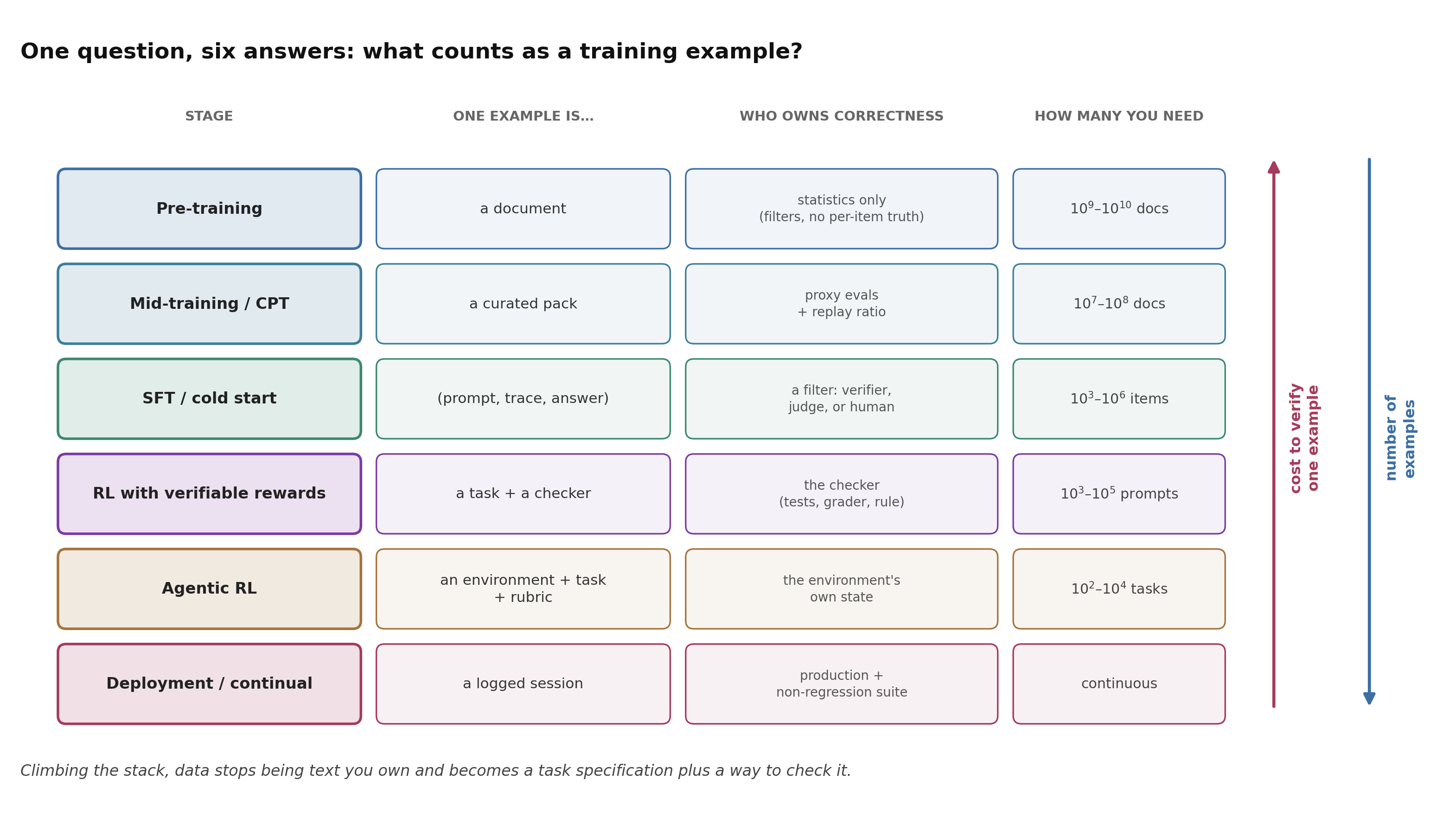 Figure 1. Six stages, six different objects called “data.” As you climb, the cost of verifying one example rises by orders of magnitude while the number of examples you need falls by orders of magnitude. Counts are typical of public recipes, not hard limits.
| Stage | One example is… | Where it comes from | Who certifies correctness | Signature failure |
|---|---|---|---|---|
| Pre-training | a document | crawl, licensed corpora, code | nobody — only statistical filters | contamination, duplicate spam, quality drift |
| Mid-training / CPT | a curated pack (domain, long-context, annealing) | up-sampled real + rewritten | proxy evals, replay ratio | forgetting, lost plasticity, recognition without recall |
| SFT / cold start | (prompt, trace, answer) | teacher distillation, self-generation, humans | a filter: verifier, judge, or human | style without substance; the teacher’s ceiling |
| RL with verifiable rewards | a task plus a checker | curated hard problems, reverse construction | the checker (tests, grader, rule) | mislabeled gold, wrong difficulty band, reward hacking |
| Agentic RL | an environment + task + rubric | environment synthesis, session replay | the environment’s own state | fake tools, unreachable goals, brittle graders |
| Deployment / continual | a logged session | production traffic | non-regression suite + users | privacy, feedback loops, silent drift |
The six stages and the six objects. The column that actually predicts your engineering effort is “who certifies correctness.”
Two consequences are worth stating before we go anywhere else.
The unit of data stops being text. In pre-training you buy tokens. In RLVR you buy problems with checkers — the answer is not the data, the checker is. In agentic RL you buy environments, which is to say you buy software. This is why data work migrates from data engineering to software engineering as you go up, and why the headcount profile of a post-training team looks nothing like a pre-training data team.
The economics invert. A pre-training corpus is 10⁹–10¹⁰ documents with essentially zero verification cost per document. An RLVR run is 10³–10⁵ prompts, each of which needs a checker that someone wrote and validated. Agentic RL is 10²–10⁴ tasks, each of which may need a Docker image. Per-example cost rises by five or six orders of magnitude while the example count falls by five or six — which is why “just get more data” is good advice at the bottom of the stack and nearly always wrong at the top.
Takeaway. “Training data” is six different objects with six different certifiers. Before answering any data question, say which stage you are in and who owns correctness there. Half of all disagreements about synthetic data are two people standing on different rungs.
Three sources of supervision
“Synthetic versus real” is the wrong axis, and it produces unresolvable arguments because both sides are describing different regimes. The axis that actually predicts behavior is who supplies the correctness signal, and there are exactly three candidates.
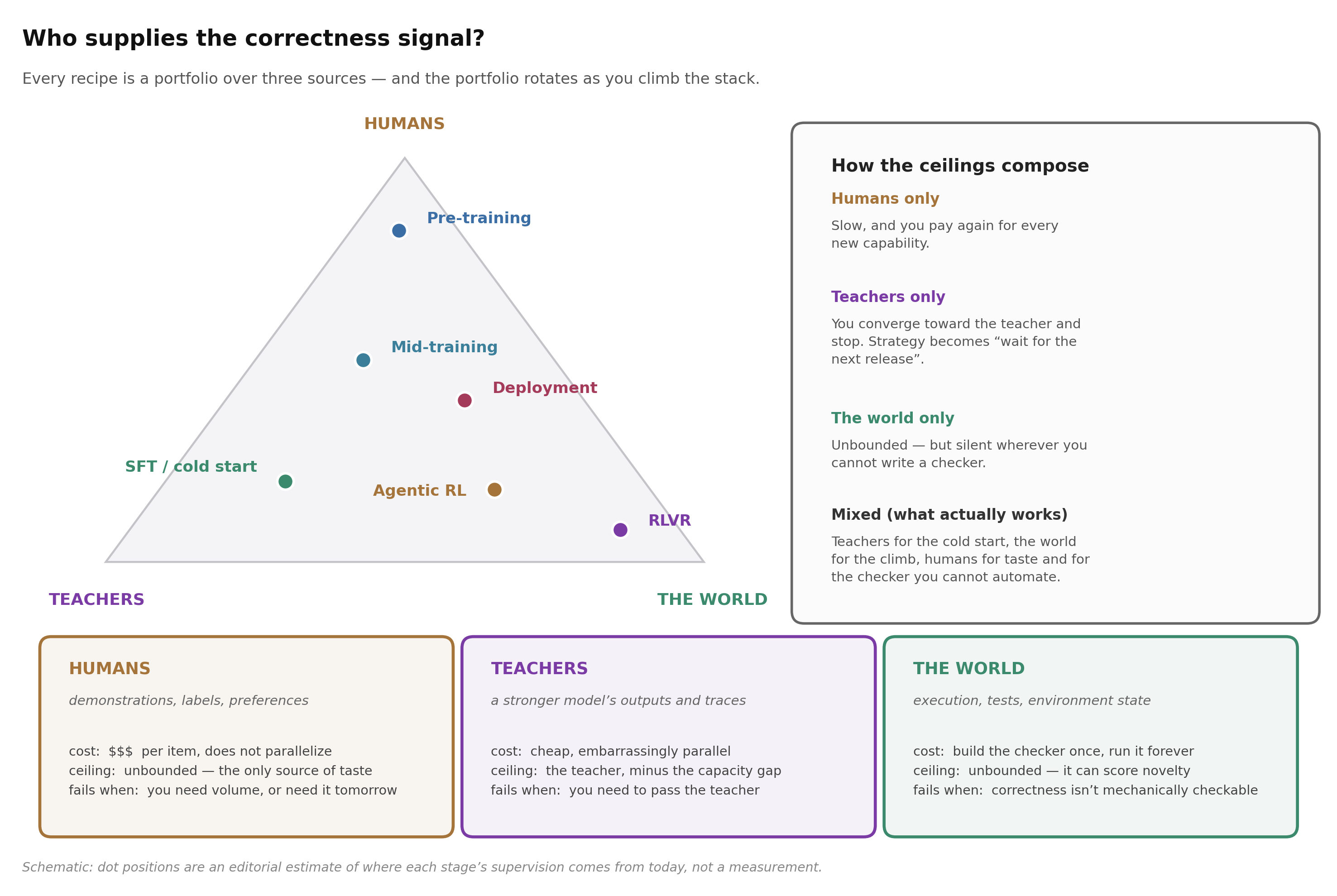 Figure 2. Every recipe is a portfolio over three sources of correctness. The portfolio rotates as you climb the stack: pre-training leans on human text, SFT on teachers, RL on the world. Dot positions are editorial, not measured.
- Humans. Demonstrations, labels, preferences, and — critically — taste. Unbounded ceiling, because a human expert can recognize quality nobody has formalized. Also unscalable, and you pay again for every new capability.
- Teachers. A stronger model’s outputs: answers, traces, trajectories, judgments, logits. Cheap, embarrassingly parallel, and available today at a price that rounds to zero next to a training run. Its ceiling is the teacher, minus a capacity-gap penalty we will quantify later.
- The world. Execution: compilers, unit tests, proof checkers, simulators, environment state, real users. You build the checker once and run it forever, and — the important part — it can score behavior nobody has produced before, which is the only property that lets a model pass its teachers. Its weakness is total: outside checkable domains it says nothing at all.
The reason to insist on this framing is that it makes ceilings composable. If every supervision signal in your pipeline comes from a teacher, your model converges toward that teacher and stops; your strategy has quietly become “wait for the next teacher release.” If every signal comes from the world, you are unbounded but silent everywhere you cannot write a checker — which today means most of what people actually want from assistants. Working recipes are portfolios: teachers for the cold start, the world for the climb, humans for taste and for the checkers you cannot automate.
The portfolio also explains an empirical pattern that otherwise looks like a coincidence. The largest, most reliable “synthetic data” wins in the literature are not synthetic text — they are synthetic labels. FineWeb-Edu had Llama-3-70B score 460k web pages for educational value, distilled those judgments into a linear head on a frozen embedder (F1 ≈ 82% at threshold 3), and applied it to 15T tokens for ~6,000 H100-hours; the resulting 1.3T-token corpus reaches 33.6% MMLU at 38B tokens where the next-best dataset needs ~300B — roughly 10× token efficiency (Penedo et al., 2024). DataComp-LM’s entire headline result is a filtering-model swap that moves MMLU from 35% to 44% at fixed 7B/280B compute (Li et al., 2024). phi-1’s first ablation, before any generated text enters, is a GPT-4-labeled quality classifier (Gunasekar et al., 2023).
Insight — the teacher’s best job is verification, not authorship. A frontier model used to write your data caps you at its distribution. The same model used to score your data multiplies the value of a corpus you already own, and the score can be distilled into something cheap enough to run over trillions of tokens. When people say “synthetic data works,” the load-bearing wins are usually of the second kind.
The synthesis playbook
Once you accept that generation is cheap, the interesting question is not whether to synthesize but which operator to apply. There are eight recurring patterns, and each one has a characteristic failure that shows up reliably enough to predict.
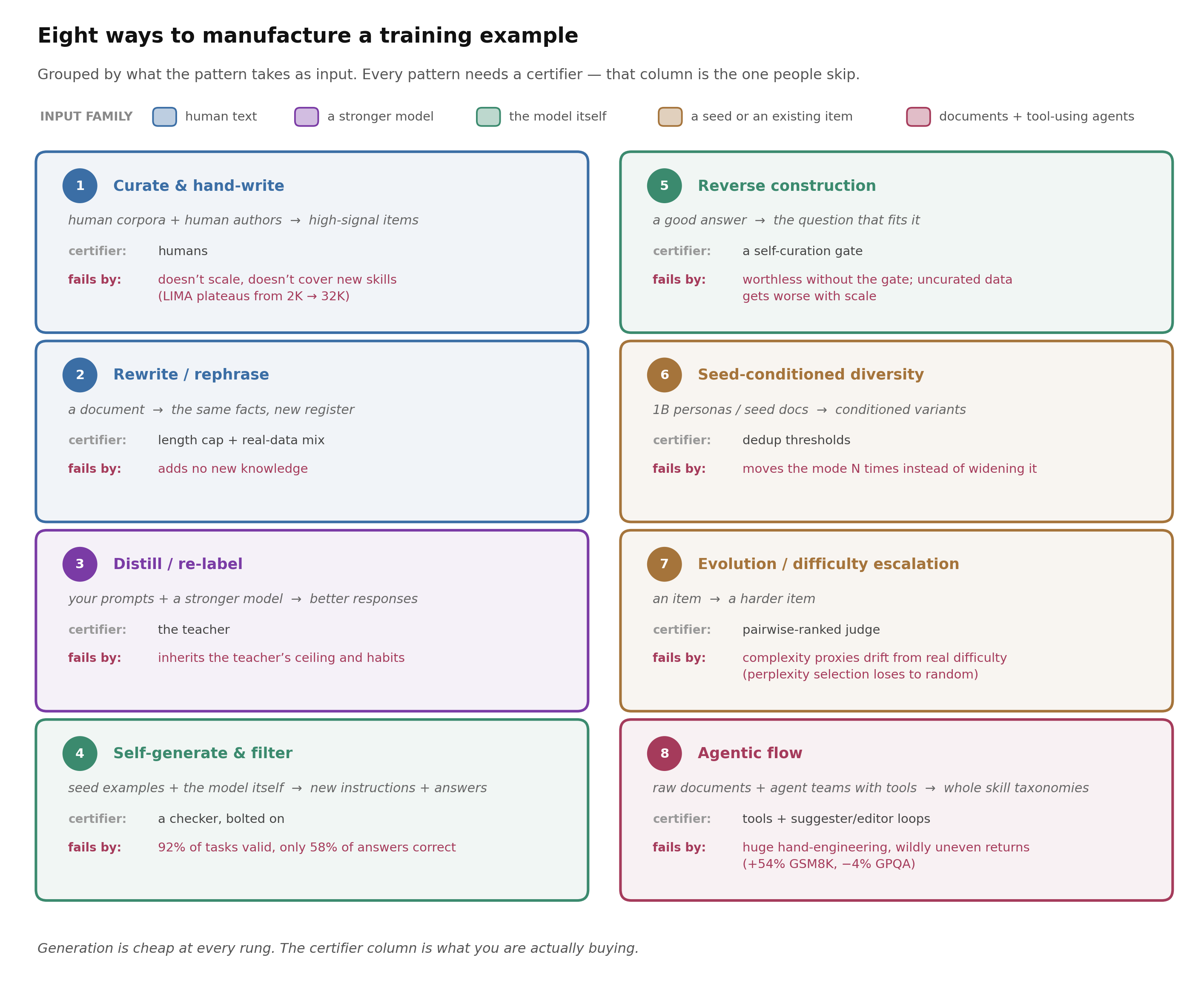 Figure 3. Eight ways to manufacture a training example, arranged by what they take as input. The right-hand column is the part people skip: every pattern needs a certifier, and the pattern only works as well as that certifier.
Eight patterns
1. Curate and hand-write. No synthesis at all: mine high-signal human corpora under hard filters, then hand-write the tail. LIMA’s 1,000 examples (750 mined from Stack Exchange / wikiHow / Reddit under explicit length and register filters, 250 hand-written) were judged equal-or-better than GPT-4 in 43% of pairwise comparisons on 300 open-ended prompts (Zhou et al., 2023). Fails by: not scaling and not covering skills. Quality plateaued from 2K to 32K examples, and reproductions on smaller bases score it far lower.
2. Rewrite and rephrase. Keep the information, change the style. WRAP has a frozen Mistral-7B paraphrase C4 documents into four registers (easy / medium / hard / QA), caps each at 300 tokens because the rephraser starts losing information beyond that, and trains on a 1:1 real:synthetic mix for ~3× pre-training speedup (Maini et al., 2024). Fails by: adding no knowledge. The paper says it outright — “synthetic data can not impart ‘new knowledge’. It can only help pre-train faster” — and its own knowledge-heavy table has TinyLlama-on-1T-real-tokens edging out the synthetic mix, 45.6 against 45.5.
3. Distill or re-label. Keep your prompts, replace the responses with a stronger model’s. The cheapest high-yield intervention in the entire SFT literature is Self-Instruct’s own ablation: regenerate only the output field with a stronger model, changing zero prompts, and the fraction of outputs given the top rating on a four-level scale goes from 44.4% to 54.4% (Wang et al., 2022). Fails by: inheriting the teacher’s ceiling, and its habits (see distillation).
4. Self-generate and filter. The model proposes, a checker disposes. Self-Instruct bootstrapped 52,445 instructions from 175 seeds with a ROUGE-L < 0.7 novelty gate. The number to remember is its audit: 92% of generated instructions describe a valid task, but only 58% of outputs are correct. Fails by: producing wrong answers. This pattern generates instruction distributions reliably and solutions unreliably, which is precisely why it needs pattern 3 or a verifier bolted on.
5. Reverse construction. Run the pipeline backwards: treat existing high-quality text as the gold response and generate the instruction that would have produced it. Humpback trains a backward model p(x|y) over 502k web segments, self-curates to 41,821 pairs with the model’s own 5-point score, and reaches AlpacaEval 83.71 at 65B from 3,200 human annotations (Li et al., 2023). Its data-scaling coefficient (win rate per log-example) is 6.95, against LIMA’s 2.86 and Alpaca’s 1.99. Fails by: being worthless without the curation gate — uncurated backtranslated data gets worse with scale.
Insight — generate the question, not the answer. Reverse construction wins because it moves the hard half of synthesis to humans who already did it. Writing a correct, well-written, factually grounded response is the expensive part; inferring a plausible question from a good answer is nearly free. The same trick reappears at every level of the stack: answer → problem for math, merged PR → issue for code, observed environment state → task for agents.
6. Seed-conditioned diversity scaling. Condition generation on a large external set of contexts so the generator cannot return to its mode. Persona Hub mines ~1.01B personas from the web via text-to-persona and persona-to-persona expansion, deduplicates with MinHash at 0.9 and embedding similarity at 0.9, and prepends one to any synthesis prompt; persona pairs at 0.9 similarity yield problems at 0.6–0.75 similarity, so the persona set acts as a diversity lower bound (Ge et al., 2024). Tülu 3 uses ~250K of them and reports that removing the persona data costs 19.2 points of IFEval (Lambert et al., 2024). Fails by: moving the mode 250,000 times rather than widening it (see below).
7. Evolution and difficulty escalation. Take an item and rewrite it to be harder, repeatedly. Deita’s key move is not the evolution but the scoring: evolve each instruction five times, then ask the judge to rank and score all six variants in one prompt, because a judge asked to grade a single example in isolation compresses everything into 7–8/10 (Liu et al., 2023). LIMO gets the same end by selection instead of generation — keep only problems a strong reasoner solves 1–3 times out of 32 (Ye et al., 2025). Fails by: complexity proxies drifting from real difficulty. In Deita’s controlled comparison, perplexity-based selection (4.06 / 1.89 MT-Bench) and instruction-length-based selection (4.00 on the noisy pool) both score below random selection (5.84 / 4.93), because high-perplexity samples turn out to be the ones with very short responses.
8. Agentic-flow generation. Decompose synthesis into stages, each a bank of role-specialized agents, some with tools. AgentInstruct seeds from raw documents and code — never from prompts — runs content transformation (nine agents for reading comprehension alone), then per-question-type generation (43 types), then Suggester–Editor pairs whose only job is to make items harder; 17 skills, 100+ subcategories, 22M pairs from the pipeline itself (Mitra et al., 2024). Giving the agents tools is the mechanism by which generated responses can exceed the generating model. Fails by: enormous hand-engineering and wildly uneven returns — the same pipeline that moves GSM8K +54% moves IFEval +2% and GPQA −4%. Read the headline number carefully, too: the commonly quoted ~25.8M is the 22M synthetic set plus 3.8M of Orca-2.5 data, so the reported gains are not attributable to the agentic pipeline alone.
Diversity is the binding constraint
The sharpest result in this entire literature is about diversity, and it reframes the synthetic-data debate. Verbalized Sampling starts from a mechanism rather than a symptom: annotators in preference data systematically prefer text with higher base-model log-probability, independent of quality. Model the reward as r_true + α·log π_ref and the aligned optimum becomes π* ∝ π_ref^γ with γ = 1 + α/β > 1 whenever α > 0. Fitting α on correctness-matched pairs gives α̂ ≈ 0.57–0.65 with p < 10⁻¹⁴. So on any subset where true quality is flat across candidates — creative writing, dialogue, most open-ended synthesis — alignment sharpens the model onto the base model’s mode, and typicality bias is the tiebreaker (Zhang et al., 2025). The derivation is airtight; what it rests on is the modeling assumption that log π_ref proxies a typicality preference, which the authors are explicit about.
The measured consequence for a data pipeline is brutal. Generate 1,000 synthetic competition-math questions from GPT-4.1 and Gemini-2.5-Flash with an ordinary prompt, have Qwen3-32B write traces, and SFT small students on the result: the average of MATH500 / OlympiadBench / Minerva comes out at 30.6, below the 32.8 you get by not fine-tuning at all. Change nothing except asking for “five responses with their probabilities” instead of one, and the same teachers, budget, and students give 36.1, rising to 37.5 for the multi-turn variant of the same prompt. The sign of the return flips on a prompt rewrite.
The same paper measures how mode collapse accumulates through post-training: on a poem task, base model diversity 45.4% → 20.8% after SFT → 10.8% after DPO, while distribution-level prompting holds ~30% throughout (Zhang et al., 2025).
Trade-off — conditioned diversity is not sampled diversity. Personas, seed documents, and topic taxonomies raise diversity by moving where the mode is, once per condition. Distribution-level prompting raises diversity by flattening the sampling distribution itself. They are complementary and, as far as I can tell, nobody has published the combination. If you run a synthetic-data pipeline off an aligned model, the second is close to free and you should check it before buying more personas.
The verification ladder
If generation is cheap and verification is the asset, then the central design decision in any data pipeline is which certifier you attach to each example — and that is a ladder, not a binary. Each rung costs more, covers more of what you actually mean, and fails in its own way.
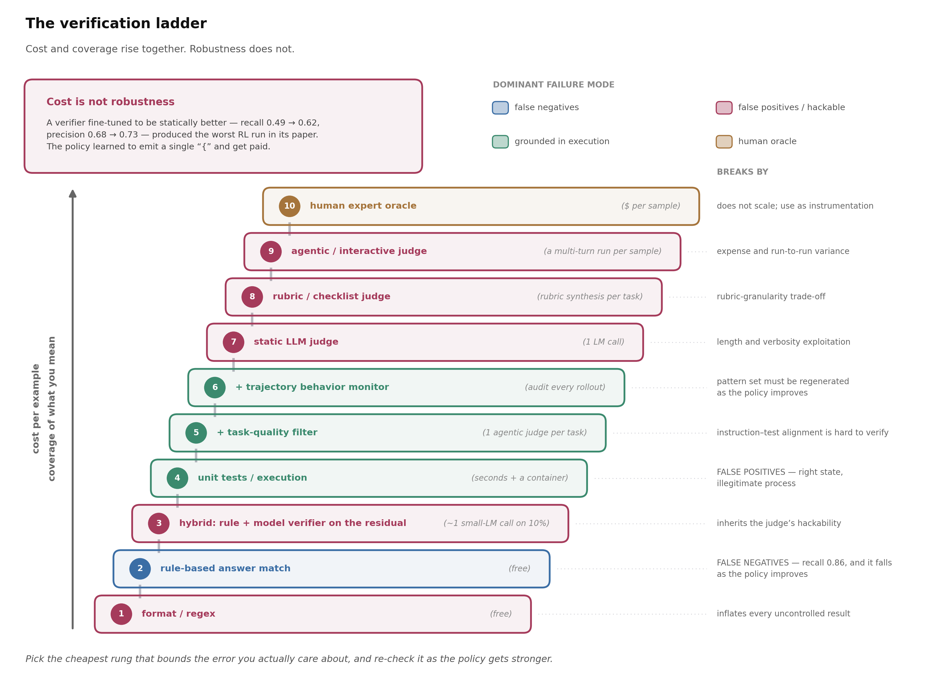 Figure 4. The ten most common verification mechanisms, ordered by cost per example and colored by the error class each one is dominated by. The rule is not “climb as high as possible” but “pick the cheapest rung that bounds the error you care about” — and note that robustness is not monotone in cost. The table below adds three rungs the figure omits.
| Mechanism | Cost | Covers | Breaks by |
|---|---|---|---|
| nothing (entropy, random reward) | free | nothing | amplifying whatever the prior already favors |
| format / regex | free | answer presence | inflating every uncontrolled result |
| rule-based answer match | free | canonical final answers | false negatives, worse as the policy improves |
| hybrid: rule first, model verifier on the residual | one small-LM call on ~10% | answer equivalence | inheriting the judge’s hackability |
| unit tests / execution | seconds–minutes + Docker | behavior the tests happen to cover | false positives: right state, illegitimate process |
| + task-quality filter | one agentic judge per task | removes tasks whose reward is meaningless | instruction–test alignment is hard to check |
| + trajectory behavior monitor | log and audit every rollout | outcome and process legitimacy | pattern set must be regenerated as the policy improves |
| static LLM judge | one LM call | subjective quality | length and verbosity exploitation |
| rubric / checklist judge | rubric synthesis per task | structured, multi-dimensional quality | rubric-granularity trade-off |
| agentic / interactive judge | a multi-turn agent run per sample | runtime behavior, whole repos | expense, run-to-run variance, role confusion |
| learned discriminator vs demonstrations | co-training a second model | distributional properties no scalar captures | adversarial non-stationarity |
| real user feedback | free at inference, costly to instrument | the actual holder of the intent | extreme sparsity and asymmetry |
| human expert / strong-model oracle | dollars per sample | ground truth, approximately | does not scale; use as instrumentation |
The verification ladder. Evidence for each rung is in the sections below; the important structural facts are that cost and coverage rise together, and robustness does not.
Three facts about this ladder are worth more than the ladder itself.
The two errors are not symmetric
Rule-based verifiers fail by false negatives. A careful audit of three standard math verifiers across four datasets found precision above 99% but recall averaging 0.86, 0.92, and 0.93 — for the weakest of the three, roughly one in seven correct answers scored wrong — dropping to 0.78 on the hardest dataset and 0.35–0.58 outside mathematics (Huang et al., 2025). The paper’s own reported trend is that recall degrades on the harder, more diverse answer distributions produced by stronger policies. Model judges and test suites fail the other way, by false positives: the reward is paid and the behavior is wrong.
Both error types get worse as capability grows, which is the real content of the phrase “verification horizon.” But they are not equally dangerous. Unbiased noise degrades; biased noise steers. One-shot RLVR experiments show 60% randomly wrong labels costing only ~1.3 average points, and even 90% wrong labels leaving the run above nothing (Wang et al., 2025) — but a wrong label the model can plausibly reach is far more damaging than one it cannot: on a single training example, a wrong-but-guessable answer scored 57.0 versus 64.4 for a wrong-and-unreachable one and ~74 for the correct one. The dangerous mislabel is the plausible one.
Grounding beats sophistication
Every robustness win in the literature comes from grounding the reward in something the policy cannot rewrite — execution, process logs, a live browser, a co-evolving discriminator, real users. Every robustness loss comes from asking a model to read and opine. The quantitative version: across 13 adversarial hacking patterns, discriminative verifiers that emit a judgment directly suffered 0.1–0.4% attack success, while generative CoT verifiers ranged 7.7–23.7%, with the worst single cell at 77.9% for a fake “answer explanation” attack (Huang et al., 2025). The chain of thought is itself the attack surface.
The most counterintuitive result in the same study is the one to remember for interviews: the authors fine-tuned a verifier to be statically better — recall 0.49 → 0.62, precision 0.68 → 0.73 — and it produced the worst RL run in the paper, because the policy discovered it could emit a single { and get paid. Static classification accuracy did not predict RL outcome, in the wrong direction.
Takeaway. Choose verifiers by adversarial robustness and by what happens over a training run, never by held-out accuracy. Two instruments make this cheap: an adversarial pattern suite, and an oracle channel — re-score ~1,000 sampled training prompts with a strong external model at every checkpoint and plot training reward against oracle reward on the same axes. Divergence between those two curves is the most reliable alarm you can buy.
Pre-training: filtering is the product
I covered the pre-training funnel — extract, deduplicate, classify, mix — in the frontier-labs post, so here I only want the parts that change how you think about the rest of the stack, plus the results that overturned received wisdom.
Model-based filtering is the highest-leverage knob anyone has measured, and “quality” means “shaped like the task.” DCLM’s controlled benchmark (five compute scales, 416 baseline experiments, 53 evaluations) found a plain fastText bigram classifier beating perplexity filters, embedding classifiers, semantic dedup, and AskLLM (Li et al., 2024). The reference corpus for the positive class mattered more than the classifier: instruction data plus r/ExplainLikeImFive beat a Wikipedia/books/OpenWebText reference set by 3.5 CORE points, and filtering hard (top 10%) beat top 15% and top 20%. The whole pipeline turns 240T raw tokens into a 3.8T-token corpus; the 7B model they train on 2.6T tokens of it reaches 64% MMLU.
The finding I would put on a poster: in the same benchmark, the AskLLM filter agreed with human annotators at ~82% ROC-AUC and produced worse models than fastText classifiers, and the correlation between annotator agreement and downstream score had R² < 0.3. The best filter is not the one that agrees most with humans about what good writing is.
Deduplication is not monotonically good. FineWeb ran iterative global MinHash across 96 Common Crawl snapshots and removed up to 90% of the oldest crawls, leaving 4T tokens with essentially no gain over not deduplicating (Penedo et al., 2024). The direct test is the memorable one: on a single 2013 crawl, the ~31B tokens that survived global dedup trained a worse model than the 171B tokens obtained by independently deduplicating the 90% that global dedup had thrown away. Being duplicated across crawls is weak evidence a page is worth keeping, so global dedup preferentially keeps ads and keyword spam. Per-snapshot dedup (20T tokens) is the recipe that works.
The unit of selection can be smaller than the document. Rho-1’s token-level census on a filtered math corpus is a permanent argument-ender: 51% of tokens are already learned, 26% are where learning happens, 11% are irreducibly hard, and 12% get worse during training. Masking the loss to the top ~60% of tokens by excess loss (learner loss minus reference loss) gives a 1B model +16.5 average points on math and lets a 7B model match a 500B-token math specialist using 15B tokens — 3% of the tokens (Lin et al., 2024).
The wall, and what repetition buys
The data-wall forecast is worth quoting precisely, because the popular version of it is wrong in both directions. The estimate for the indexed web is ~510T tokens; quality adjustment (only 10–40% is usable) takes that to a median 100T; repetition adjustment takes it back to ~320T. Demand grows ~0.38 OOM/year (2.4×/year), and the median crossing is 2028 (Villalobos et al., 2022). Anyone saying “the web is huge, we’ll never run out” is quoting the raw number; anyone saying “we ran out last year” is ignoring repetition and the fact that filters keep improving.
How much does repetition buy? The canonical answer: up to 4 epochs is nearly free (an 8.7B model trained 4 epochs on 44B unique tokens ends 0.5% worse in validation loss than one epoch on 178B unique tokens), meaningful gains continue to ~16 epochs, and by 40 epochs repeating is worthless. The fitted half-lives are the part people forget: repeated tokens decay in value with R*_D = 15.4 while excess parameters decay with R*_N = 5.3, so when you are data-constrained you should buy epochs before parameters — the opposite of Chinchilla’s equal split (Muennighoff et al., 2023).
Open question — the 4-epoch rule is model-size-dependent. A 2026 study fixing the repetition confound found the optimal number of passes over a scarce high-quality corpus ranges from ~24 for a 30M model to ~5 for a 757M model, with the optimal high-quality share falling from 0.75 to 0.15 over the same range (Repetition Mismatch). Bigger models want fewer repetitions and more fresh web text. “Four epochs” is a number from one scale, not a law.
Collapse is a protocol bug
The model-collapse literature is usually cited as a reason to fear synthetic data, and the citation is almost always to the wrong claim. The original result proves that recursively training on your own outputs while replacing the previous data collapses the distribution to a delta function, and demonstrates degradation on a 125M model fine-tuned on 2M words (Shumailov et al., 2023). But that paper’s own condition where 10% of the original data is preserved each generation already shows “only minor degradation.”
Make the protocol match reality — data accumulates on the web, it is not swapped out — and the divergence disappears. Under accumulation, test error is provably bounded by a constant independent of the number of iterations (σ²d/(T−d−1) · π²/6), versus linear divergence in the number of generations under replacement; empirically, cross-entropy stays flat over five iterations for every model size tested (Gerstgrasser et al., 2024).
Takeaway. The operational rule is never replace, always accumulate, and the question to ask is not “is synthetic data poison?” but “what fraction of this corpus is real, and does it stay in?” Note the honest version of the good news: the accumulation bound is
π²/6 ≈ 1.645×the single-iteration error, a real 64% penalty, and the collapse experiments I could find all run at ≤126M parameters. Nobody has published a frontier-scale test.
Why mixture experiments lie
Mixture optimization is where the field’s methodology problem is most visible. The appealing assumption is rank invariance: if mixture A beats B on a small proxy, it beats B at target scale. Three independent 2026 results say that assumption fails, each for a different reason.
The confound: because a scarce high-quality corpus is repeated a different number of times at proxy budget than at target budget, the loss landscape moves. Hold repetition fixed by subsampling the datasets as well as the horizon and a single proxy run at 6% of the target token budget lands within 0.05 of the optimal mixture, versus 0.75 error for naive extrapolation — and matching that accuracy without the correction costs 44–94% of the full budget (Repetition Mismatch).
The mechanism: the optimal training mixture is genuinely not the target mixture and genuinely moves with model size and token count. A mechanistic model with capacity competition plus a data-driven noise term fits 64 existing runs with ~85 free parameters and, fitted only at 122M/10B, extrapolates a 1B/30B mixture that matches an empirical law fitted with access to the target scale (Dai and Zheng, 2026).
And the sanity check: DoReMi — the method that made proxy-based mixture optimization standard, with +6.5pp downstream on the Pile (Xie et al., 2023) — loses to uniform in three of four pairings when the domains are 256 learned semantic clusters instead of 22 provenance labels, plausibly because a worst-group objective up-weights format-heavy junk that no capability benchmark rewards (Qiao et al., 2026).
Insight — granularity and the selection rule are jointly determined. The same study found per-bucket quality selection worth +0.025 at 65k buckets and worth nothing at 130k, because the median candidate pool contracts from 2,271 documents to 429 and within-bucket ranking degenerates toward a uniform draw. Finer domains help until your buckets are too small to rank inside. This is the same shape as the difficulty-band problem in RL: selection needs a population to select from.
Mid-training: the stage nobody writes down
Mid-training is the stage with no agreed definition, no canonical recipe, and — not coincidentally — the most interview questions. Operationally it is everything that happens after you decide pre-training is finished and before you start collecting preference or reward data: up-weighting a domain, extending context, annealing on a high-quality mixture, installing an output format, injecting a proprietary corpus, and preparing the model so that RL has something to amplify. Tech reports mention it in a sentence. It is also, for most people reading this, the only stage where a modest budget can still move a frontier-adjacent number, which is exactly why it gets asked about.
The unit of data here is a curated pack, and the certifier is the weakest of any stage: a proxy eval plus a replay ratio. Nobody checks individual documents. What you are actually deciding is a distribution and a schedule, and the recurring lesson across the literature is that the same facts in a different format are worth roughly an order of magnitude more. Mid-training is the one stage where you can change what a training example looks like without changing who supplies correctness.
Continual pre-training mechanics
There is a stable knob set, and it is small enough to memorize.
| Knob | Setting | Evidence |
|---|---|---|
| Checkpoint | the most converged one you have; better still, a non-decayed checkpoint | later checkpoints won at every budget tested (Gupta et al., 2023); DeepSeek-V2 resumed pre-decay to skip re-warming |
| Warmup length | a non-decision — use ~1% to suppress the initial spike | 0%, 0.5%, 1%, 2% converge to the same loss (Gupta et al., 2023) |
| Peak LR | ~5e-5 for an 8B-class model on tens of billions of tokens | (Zhou et al., 2026); every production recipe below lands near it |
| Decay | cosine to 0.1× peak | (Ibrahim et al., 2024) |
| Replay | 1–5% weak shift, ~25% strong shift, 30–60% in production runs | (Ibrahim et al., 2024) |
| Mixture | always mixed, never domain-by-domain; keep ~1% instruction data | domain-incremental CPT degrades (Ibrahim et al., 2024); ~1% instruction (Wang et al., 2025) |
| Budget | ~15–27B tokens for capability work; more if RL follows | (Runwal et al., 2026); (Wang et al., 2025) |
The continual-pre-training knob set. Only two of these are genuinely contested: peak LR and replay.
Roughly a third of what people call catastrophic forgetting is the learning-rate schedule, not the data. Re-warm and re-decay a 405M model on the very Pile data it was pretrained on and Pile validation loss still rises by a peak of +0.1 nats at η_max = 3e-4 and +0.2 at 6e-4. With a real shift to SlimPajama the peaks are +0.35 and +0.45 — so the schedule accounts for something like a quarter to a half of the observed regression, and models “fail to recover quickly from the performance hit even when training on the same dataset” (Ibrahim et al., 2024). Before you blame the new corpus, price in the optimizer. This is also the entire motivation for infinite-LR schedules and for resuming from a non-decayed checkpoint.
Set the replay ratio by the size of the distribution shift, not by the token budget. The numbers are unusually clean (Ibrahim et al., 2024). Pile → SlimPajama at 405M: 0% replay costs 0.27 nats on Pile; 1% replay recovers 0.18 of that at a cost of 0.00 nats on the new data (SlimPajama loss 2.50 either way). Pile → German needs 25% to reach the union-baseline average loss of 1.75, where 1% only reaches 1.97. Scale barely changes the calculus — 5% replay recovers 0.19 nats at 10B and 0.21 at 405M, because bigger models forget less to begin with. Production runs are more conservative than the papers: Zamba used 60% replay in its decay phase and DeepSeek-V2 used 30% across 6T CPT tokens. If you do not have the original pre-training data, the practical substitute is to keep a general web stream in the mixture and call it replay by another name.
The peak-LR disagreement is worth understanding rather than resolving. The canonical CPT papers (Gupta et al., 2023; Ibrahim et al., 2024) say re-warm to O(η_max) of pre-training and use η_max as your adaptation-versus-retention dial, which gives 3e-4 at 405M. A 2026 scaling study says the optimum shrinks with total effective compute, and predicts 5e-5 for a dense 8B model continuing on 55B tokens — with 5e-4 costing 3.7 average points and dropping GSM8K from 40.7 to 31.1 (Zhou et al., 2026). Both are right for their regime, and the reconciling quantity is the ratio of your CPT budget to the checkpoint’s equivalent pre-training compute, which you can estimate by measuring the checkpoint’s loss on your CPT validation set and inverting the loss–compute law. The canonical setting has 300B tokens of CPT on top of 300B of pre-training, so a high LR is correct there; a well-trained 8B model seeing 55B new tokens is a completely different point on that curve. Note also that the same study finds optimal batch size rising with compute, and rising 2.2× faster for MoE than dense — routing destabilizes at small batch.
Knowledge injection: recognition is not recall
Here is the result I would use to open any discussion of domain adaptation, because it kills the default plan.
A model can memorize a document perfectly, token by token, and be unable to answer a single question about it. Pre-train on 100,000 synthetic biographies in one fixed format, then fine-tune a QA head on half the people. Mean accuracy on the held-out half is 9.7%, against a majority-guess baseline of 2.7% — per-attribute, 33.5% on birth date (always the first attribute after the name) and 1.1–13.8% on the other five. Scale does not rescue it, and neither does effort: a 682M-parameter model — about 6,800 parameters per person — trained for 1,350 passes reaches 99.0% first-token accuracy on the QA pairs it was fine-tuned on and 4.4% on the held-out ones, and LoRA plus full fine-tuning across roughly thirty settings all fail (Allen-Zhu and Li, 2023).
The probing analysis explains why, and the explanation generalizes. In a single-format corpus the attribute is encoded diffusely across the document’s tokens rather than linearly in the hidden state adjacent to the entity’s name. A question supplies only the name. There is nothing there to read. Fine-tuning cannot fix it because fine-tuning cannot relocate where knowledge is stored — that is a pre-training-time property of the corpus.
Augmentation relocates it, and diversity rather than volume is the active ingredient. Five distinct rewrites plus sentence permutation take the same model from 9.7% to 96.6%, and probing accuracy rises in lockstep. But five rewrites in a fixed order reach only 41.0%, and permutation alone actively hurts (4.4%, worse than doing nothing). Two further properties make this operational:
- It is contagious. Add a disjoint set of 100k augmented “celebrity” biographies, fine-tune the QA task only on celebrities, and the untouched, un-augmented “minority” set goes from 4.4% to 86.8%. The model learns the storage convention and applies it to documents it saw once. You do not have to augment everything.
- There is a cheaper door. Mixing QA-format data into pre-training rather than saving it for SFT reaches 86.6% on completely un-augmented biographies.
The budget arithmetic comes from the same group. A sufficiently trained transformer stores about 2 bits of knowledge per parameter — a 7B model holds ~14B bits, which the authors estimate exceeds English Wikipedia plus textbooks — but “sufficiently trained” means roughly 1,000 exposures per fact; at 100 exposures you get 1 bit per parameter (Allen-Zhu and Li, 2024). So “make each fact appear more often, in more forms” is not a trick, it is the direct lever on the storage constant. Two corollaries worth carrying into a design review: int8 quantization is free (still 2 bits/param) while int4 collapses to 0.7; and dilution depends entirely on what kind of junk it is. Mixing in 7/8 high-entropy junk — random facts that never repeat — costs 20× capacity at 100 exposures. Mixing in 7/8 repetitive junk costs nothing. And the mitigation is almost free: prepend a provenance token to the useful documents and the 20× penalty becomes 2×, matching the no-junk law entirely by 300 exposures. The model learns to route its own capacity by domain with no prior about which domains are good.
Insight — this is why replay is not dilution. Two results that look contradictory — “7/8 junk costs 20× capacity” and “heavy replay costs almost nothing in loss” — are reconciled by the junk taxonomy. Replay data is repetitive, in-distribution, and previously learned. It is the free kind, in the sense that matters here: it does not consume capacity. What it does consume is budget — at 50% replay you see 150B fewer new tokens, which is why published recipes sit at 1–25%. High-entropy unlearnable text is the expensive kind. If you cannot clean your corpus, tag it: provenance tokens recover most of the loss for essentially no cost.
The production version of this advice is EntiGraph, and it says paraphrase is not enough. Take 265 obscure books totalling 1.3M tokens — a corpus 10,000× smaller than the smallest published domain-adaptive CPT corpus — extract entities, then ask a teacher to analyze the relations among every entity pair and triplet, always conditioned on the source document. That inflates 1.3M real tokens into 455M synthetic tokens, and CPT on them (Llama-3-8B, 2 epochs, 10% replay, peak LR 5e-6) takes closed-book accuracy from 39.49% to 56.22%, log-linear in synthetic tokens across three orders of magnitude, with a fitted asymptote of 64.5% (Yang et al., 2024). Two comparisons carry the argument:
- CPT on the raw 1.3M tokens scores 38.15% — below the 39.49% base model. Training on your own documents made the model worse.
- Rephrase CPT flattened by 38M tokens and was abandoned. Surface variation is not the same operator as combinatorial coverage of a relation graph.
And it buys most of what retrieval buys: RAG on the base model reaches 60.35 with 99.63 Recall@8, so EntiGraph’s +16.73 is 80% of RAG’s absolute gain with no test-time corpus access, and the two compose to 62.60. That is the number to have ready when someone asks whether to fine-tune or retrieve. The honest framing is the authors’ own: EntiGraph “does not create knowledge de novo; it rearranges the knowledge of the source into a layout more amenable to learning.”
A caveat I can give from the inside. Some years ago I worked on a smaller-scale version of this question, comparing question-shaped synthetic representations across all three injection routes (Zhang et al., 2024). The transferable finding is that the best data format differs by route: short aligned QA pairs for SFT, question-plus-context blocks for CPT, question-augmented articles for retrieval — and finer conditioning windows beat coarser ones. The finding I would report more carefully than the paper’s abstract does is the magnitude. The headline “+21.2% BioASQ” is an absolute F1 gain over the base model; against the right baseline — CPT on the raw articles — the gains are +11.6 / +3.1 / +1.1 F1 points on the three datasets, and on one of them raw-article CPT already achieves 0.242 of the best 0.253. That experiment was also QLoRA on thousands of examples, not full-parameter CPT on billions of tokens. Which brings up the contradiction worth knowing: in our setting raw-document CPT clearly helped, and in EntiGraph’s it was worse than the base model. The likely reason is corpus obscurity. EntiGraph deliberately chose a corpus the base model did not know; benchmark knowledge bases derived from Wikipedia and PubMed are plausibly already in pre-training, which makes “raw CPT” a refresher rather than an injection.
Trade-off — paraphrase suffices for lookup, not for comprehension. Five template rewrites take single-hop attribute extraction from 9.7% to 96.6%; the same operation on real prose flattens after 38M tokens when the questions require reasoning across a 5,000-token document. Both literatures agree diversity is the mechanism. They disagree about how much of it paraphrase supplies, and the discriminator is whether the missing representation is an attribute attached to an entity or a relation between entities. Diagnose which one you need before choosing your augmentation operator.
Long-context data is manufactured
Long-context ability is mostly unlocked, not installed: the capacity to use information at arbitrary positions is largely acquired during short-context pre-training, which is why 5B tokens does what earlier efforts spent 400B on. Needle-in-a-haystack accuracy against CPT tokens: 100M → 37.8, 300M → 59.0, 500M → 81.1, 1B → 85.3, 5B → 88.0, 10B → 84.0. The authors read the 10B dip as overfitting to the training range; it is one sweep on one model, so treat the peak’s location as approximate and the plateau as the robust part (Fu et al., 2024). The whole run is five days on 8×A100, and training at 80K context is only 3× slower per token than 4K because I/O dominates and hides the quadratic attention.
The most useful methodological result in this literature is that loss is blind to it. Two SlimPajama mixtures differing by ≤0.01 nats in validation loss at every length from 1K to 128K differ dramatically on retrieval (Fu et al., 2024). Worse, perplexity can point the wrong way: as the long-data fraction goes from 20% to 100%, PG19 perplexity keeps improving while the downstream long-task average falls (Gao et al., 2024). And the standard benchmark saturates — a model scoring 100 on needle-in-a-haystack scores 23.1 on HELMET re-ranking against Llama-3.1-8B’s 37.0. If you take one thing from this subsection: never validate a long-context recipe on perplexity or NIAH.
The two recipes on offer disagree, and the disagreement is instructive rather than resolvable:
| Preserve the mixture (Fu et al., 2024) | Curate long sources (Gao et al., 2024) | |
|---|---|---|
| Long data | upsample ≥4K docs within each domain, 30% → 70% | 30% code repos + 30% books + 3% textbooks |
| Short data | unchanged by construction | 37% curated ShortMix, treated as a first-class decision |
| Argument | targeted upsampling hurts other domains (Book↑ costs +0.029 nats on GitHub) | whole-repo concatenation is the only source with ~99B tokens ≥64K |
| Result | NIAH 88.0 at 7B, 90.0 at 13B | HELMET@128K 49.4, level with a 70B model, on 40B tokens |
Two long-context data recipes. The second reports beating the first on both long and short tasks, but it also uses a newer base model, a better benchmark, and a data source that did not exist for the first.
Three findings from the curated-source side are counterintuitive enough to be worth memorizing. 100% long data is worse than 60% long data even for long tasks, and the damage shows up after SFT — a model specialized on long documents is a poor initialization for generic instruction tuning. Train longer than you evaluate: from a 20B-token 64K checkpoint, spending 4B more tokens at 512K beats spending them at 64K when measured at 64K (recall 98.5 vs 95.0, re-ranking 32.9 vs 28.0), because a document of length nd contains (n−1)(d−1) more distance-d dependencies than n documents of length d. And the short component decides your math scores: the same long mixture with a curated short stream containing OpenWebMath and Tulu-v2 gets GSM8K 46.6, above the base model’s 44.7, where SlimPajama, FineWeb-Edu, and DCLM-Baseline all land around 39–42. One more negative result from the same work, which contradicts what several frontier recipes do: adding synthetic long instruction data to SFT hurt — 55.7 at 0%, 54.1 at 1%, 43.3 at 50%, with every fraction losing to 0% even though the intermediate points are not a clean monotone curve — and it persisted with a 70B generator.
If you mid-train at short context, assume the long context is gone. Twenty-seven billion tokens of 8K-context capability mid-training took one model’s RULER score at 128K from 59.09 to 6.46 while improving RULER at 8K to 89.02. The best repair found is oddly specific and worth remembering: merge 15% of the base weights back into the mid-trained model, then run ~1k steps of full-parameter long-context extension, which recovers 128K to 42.16 while leaving math at 44.48 and taking code from 10.71 to 25.54 (Runwal et al., 2026). Merging alone gets 11.32; extension alone gets 36.32–38.41. Alternatively, mid-train at 16K instead of 8K: in the same study’s 3B ablation, 16K beats 8K on all five benchmarks and is the authors’ recommended balance, though 32K edges it out on three of them (GPQA 39.89 vs 38.89, LiveCodeBench 14.93 vs 12.19, MATH500 82.70 vs 82.47) and loses on AIME24 (30.98 vs 31.82).
Mid-training as RL preparation
This is the framing that makes mid-training a first-class stage rather than a cleanup step, and it answers a question people ask constantly: why does R1-Zero-style RL work on some open base models and fail on others?
It is not the RL algorithm; it is the base model’s pre-training. Under GRPO, a Llama-3.2-3B base runs its response length to the 4,096 cap, opens with \boxed{}, and degenerates into repeated “Solution” statements, while a Qwen2.5-3B base grows length smoothly. Two hundred billion tokens of math mid-training at constant LR plus a 20B-token decay branch closes the gap: MATH500 goes from 7.4 (base) and 10.0 (base + RL) to 25.8 (mid-trained) and 65.2 (mid-trained + RL), against Qwen2.5-3B’s 66.4 (Wang et al., 2025). What mid-training installed was not mathematics; it was a parseable output format, enough instruction-following that the policy does not degenerate, and a corpus good enough to sample correct solutions from.
Four transferable rules come out of that work and its successors:
- Corpus quality dominates corpus size. At an identical 20B-token budget, MegaMath-Web-Pro produced large post-RL gains while FineMath-4plus reproduced the length-explosion failure.
- Distributional alignment beats volume for the QA component. Web-derived QA gave zero post-RL improvement over web-only; QA derived from the actual benchmark distributions worked. The optimal QA fraction in the decay stage plateaus at 30% and diminishes by 40%.
- About 1% instruction data is load-bearing. An 89:10:1 web:QA:instruct ratio unlocks the QA data’s benefit after ~200 RL steps and smooths length growth.
- Base evals are the wrong selection criterion. The 70B and 100B mid-training checkpoints score the same on base benchmarks and rank 100B > 70B > 20B monotonically after RL.
The weight-level evidence is the part that changed how I think about the whole pipeline. Across seven base models from four families, mid-training moves more than 90% of parameters by at least 1% (normalized L2 distance 0.175), while RL moves about 5% (L2 0.0003 — 580× smaller), leaves >93% of weights within 1% of their mid-trained values, preserves representational geometry at CKA > 0.998, and concentrates most of its change in the first 200–400 steps (Runwal et al., 2026). RL applies roughly the same weight footprint whether or not mid-training happened — it just only works if it did. The direct consequence for data planning: you cannot add a domain at RL time. Switching the RL mixture from math+code to math+code+science moved the six-benchmark average by −0.21; switching the mid-training mixture did the same thing for +5.60 average and +17.34 on GPQA-Diamond. Math-only mid-training actually lowered GPQA by 5.2 points, and adding science recovered +10.10 without costing code.
There is also a specific and unusually elegant answer to “what should a mid-training example look like if RL comes next.” Not (question, solution) but (question, a set of verified-correct but strategically different solutions). The argument starts from the gradient: one policy-gradient step changes the sampled token’s probability by about ηAε² when the model is confident, versus ηA·(1/N)(1−1/N) when mass is split across N modes — an over-confident model is nearly immovable by RL. Training on n verified-distinct solutions per question produces exactly those multi-modal branch points (RRV et al., 2026). The empirical details are what make it usable:
- Set n ≈ your RL rollout group size. With group size 16, n = 16 beat n = 64, because a group of 16 rollouts can cover 16 learned strategies but only a subset of 64.
- Depth beats breadth at fixed budget. 463 questions × 16 approaches beat 7,408 questions × 1 approach by roughly 7% relative on post-RL pass@k.
- RL composes strategies it was never shown. The fraction of chains exhibiting more than one distinct solution heuristic goes from 23.3% after mid-training to 56.7% after RL, and specific combinations that appear at 0% before RL show up at 13–37%.
- Verification is non-negotiable. The same diverse chains with incorrect final answers push post-RL pass@k below vanilla RL at every k. Diversity without a correctness filter has negative value.
- Self-generated beat distilled on the same task: 16 chains per question sampled from QwQ-32B scored lower on a diversity metric (10.95 vs 13.81) and produced more verbose, repetitive RL rollouts.
Takeaway. Mid-training is where you decide what the model can do; RL only decides how reliably it does it. Budget accordingly: ~15–27B tokens at 16K context, LR ~5e-5 cosine to 0.1×, replay set by shift magnitude, ~1% instruction data, every domain you will ever want represented, and a separate long-context repair stage afterwards. Then judge the checkpoint by post-RL performance, not by its own benchmark scores — the two decouple, and that decoupling is the single most expensive mistake available at this stage.
Two supporting decisions round out the stage. Selection: in a heterogeneous mid-training mixture the quality axis is a property of the source, not of the corpus, and any global scorer will silently delete a capability — perplexity and n-gram-importance filters collapse on long records, and DataMan cannot score them at all because of an input-length limit, so it has no signal whatsoever for agent trajectories. Thresholding within source groups halved a 50B-token corpus with no macro-average loss, but note that random sampling with source preservation is a very strong baseline (63.23 versus 64.20) and beat three of the four published filters they benchmarked, perplexity and n-gram importance and DataMan among them (MIRA). Objective routing: the loss function itself can vary with the data. On identical corpora, plain LM loss beats distillation loss on reasoning while distillation loss wins on retrieval and plausibility, and the discriminating statistic is not teacher confidence but teacher–data alignment — how much teacher probability mass sits on the token actually observed. On code the teacher already puts 83% of its mass there, so distillation only dilutes the signal; on general text it puts 50%, and the other half carries information (Yuan et al., 2026). Route by domain and you beat both single objectives. This is the cleanest quantitative statement of a theme that returns in the distillation section: a teacher helps where it agrees with reality and hurts where it merely sounds confident.
SFT: a readiness gate, not a capability source
One SFT example is a triple: a prompt, an optional reasoning trace, and a response. The certifier is whatever filter you put in front of it — a verifier, a judge, or a human. That makes SFT the stage where the certifier is most obviously a design choice rather than a property of the world, and it is why the same nominal recipe produces wildly different results in different hands.
“How much SFT data do I need” has no answer until you name the base model and the breadth of the eval. This is not a hedge; it is the single largest effect in the literature. Take 800 curated long-reasoning examples and fine-tune two 32B models from the same vendor a generation apart — Qwen1.5-32B-Chat and Qwen2.5-32B-Instruct — and AIME24 goes to 9.2% on the older base and 63.3% on the newer one. A 54.1-point swing from the base model alone, larger than any data intervention in any paper I read for this post (Ye et al., 2025). Eval breadth explains the rest of the disagreement. On a single open-ended chat metric, quality plateaus by ~2K examples and 16× more data buys nothing (Zhou et al., 2023). On a 12-skill average built from deliberate gap-filling, performance is still improving at 939,344 examples (Lambert et al., 2024). Both are true. Narrow evals saturate early because a narrow eval measures a behavior, and behaviors are cheap.
How cheap is worth internalizing, because it reframes the whole stage. Thirty multi-turn examples took a model from 45.2% “excellent” responses to 76.1% and dropped dialogue failures from 15 of 42 turns to 1 of 46 (Zhou et al., 2023). Six examples were enough to install reliable structured output. The unit of SFT data is not an example, it is a behavior, and a behavior costs single to double-digit examples on a base model that already has the underlying capability. What it cannot buy is the capability itself — which is the bridge to the distillation section, and the reason the correct mental model for SFT is a readiness gate: it decides whether the model can be asked for what it already knows, and whether RL will have a usable policy to improve.
The axes are ordered, and the order is not the one people argue about. “Quality versus quantity” is a badly posed question; the evidence supports a strict precedence:
- Correctness is a gate, not an axis. In verifiable domains, wrong data has negative value. A 100K-example uncurated math-reasoning corpus — NuminaMath, an external dataset — scored 32.3 against the un-fine-tuned base model’s 49.9, so 17.6 points of damage from training (Ye et al., 2025). Eight hundred curated examples on the same base and the same eval suite scored 78.1.
- Then prompt diversity, because it sets the ceiling. At equal response quality and equal count, diverse prompts beat homogeneous ones, 3.83 versus 3.49 on a 1–6 scale (Zhou et al., 2023). With complexity and quality held constant, diversity-based selection alone moves MT-Bench 5.82 → 6.17 (Liu et al., 2023). And the largest single-ablation drop in the most thoroughly ablated open recipe is removing the persona-conditioned data that exists only to inject diversity: −19.2 IFEval points, against −12.1 GSM8K for removing all the math data (Lambert et al., 2024).
- Then response quality, because it sets the slope. Regenerating only the response field with a stronger model, changing zero prompts, moved the top-rated fraction from 44.4% to 54.4% (Wang et al., 2022).
- Then quantity, which is only free once the first three hold. Curated backtranslation gains 6.95 win-rate points per log-example against 2.86 for hand-curation and 1.99 for Alpaca (Li et al., 2023) — everything scales, but curated-and-diverse data scales 2.4× faster.
Most published selection signals are worse than random, and the failures rhyme. In one controlled comparison at a fixed 6K budget on the same pool, perplexity-based selection scored 4.06 and 1.89 on two pools where random scored 5.84 and 4.93; instruction-length selection scored 4.00 on the noisier pool, below random there, and only drew level on the other; but response-length selection scored 5.65, above random (Liu et al., 2023). Length is informative on the output side and misleading on the input side, and high perplexity turns out to select for very short responses. The signals that do work share a structure: they compare candidates against each other rather than scoring them in isolation. Asking a judge to rate one instruction’s complexity compresses everything into 7–8/10; evolving that instruction five times and asking the judge to rank and score all six variants in one prompt produces real discrimination (6.27, against 5.16 for direct scoring — though that pairs a full-pool number against a 50K-subsample one; matched at 50K it is 5.73). The same principle explains why the strongest reasoning-data selector is not a judge at all but a measurement: keep problems a strong reasoner solves 1–3 times out of 32. Changing only which problems you select, holding the solution source fixed, was worth +16 points on AIME24 (Ye et al., 2025).
Insight — score in families, not in isolation. Every reliable data-selection signal in this literature is relative: rank six evolved variants against each other, measure a solve rate across 32 samples, compare embedding distance to already-selected neighbors. Every unreliable one is absolute: rate this example 1–10, take its perplexity, measure its length. If you are building a data scorer and it takes one example as input, expect it to underperform random selection.
Two honest caveats before leaving the stage. First, the “less is more” results are compute-efficiency results more often than performance results — even the paper arguing for 800 examples reports its best numbers at its largest dataset size (2,000). Second, SFT sharpens more than it broadens, and this matters if RL comes next: a self-taught-reasoner-style SFT pass gained +1.94 on pass@1 and nothing at pass@64, while mid-training on multiple verified solutions per question gained on both (RRV et al., 2026). If your SFT stage is a cold start for RL, evaluate it at pass@k, not pass@1, because pass@1 is exactly the metric that rewards collapsing the distribution you are about to ask RL to explore.
RL data is prompts, not answers
The single most common misunderstanding about RL data is that it is a dataset of correct answers. It is not. An RLVR example is a task plus a checker, and the answer — if it exists at all — is an implementation detail of the checker. This changes what you shop for. You are no longer buying responses; you are buying problems with the property that success is mechanically detectable, which is a much rarer and more expensive object.
The first-order property of a good RL prompt is that it produces reward variance. With a group-normalized advantage, a prompt where every rollout scores the same contributes literally no gradient, so a pass rate pinned at 0 or 1 is wasted compute. The two published selection criteria I know of are both operationalizations of this — and the authors of the second are explicit that their criterion “is not necessarily optimal” and is not the load-bearing part of their result: one scores each prompt by how closely its per-epoch reward trajectory tracks the average learning curve and keeps the 16.3% that align best, matching full-set performance and beating a random subset of identical size by 8.7 average points (Li et al., 2025); the other simply keeps prompts with high historical reward variance (Wang et al., 2025).
Being unsolvable is worse than being absent. This is the asymmetry to remember. In the one-example study, training on a problem the model never solves drove MATH500 to 45.0 — below the 65.6 you get from a format-only reward, and barely above the base model. A zero-pass-rate prompt is not “hard data”; it is either genuinely out of reach, mislabeled, or unverifiable, and those three demand completely different responses. Never-solved buckets are systematically enriched in broken tasks (Verification Horizon), so “filter to the hardest examples” as a slogan will quietly fill your training set with garbage. The related finding: prefer whole problems to their hard sub-steps. Reducing a problem to just its difficult arithmetic step dropped the average from 35.0 to 30.0 (Wang et al., 2025), because the chain-of-thought around the hard step is part of the training signal.
And the amount of prompt data needed is smaller than anyone expected, in a way that should make you suspicious. One training example reached a 35.7 six-benchmark average against 35.9 for the 1,209-example set containing it. Training accuracy on that single problem saturates before step 100 while test accuracy keeps rising for another 1,400–1,900 steps — post-saturation generalization, and the model does not overfit until millions of rollouts on one problem.
That result, and a companion one, force a question you should ask about your own runs.
Is your RL teaching or eliciting? On Qwen2.5-Math-7B, RLVR with random rewards — a coin flip — gains +21.4 points on MATH-500 against +29.1 for ground-truth rewards, which is 73% of the entire supervised gain reproduced by noise. Deliberately incorrect rewards gain +24.1. The mechanism is identified rather than asserted: the clipping term in GRPO asymmetrically favors already-likely tokens, so the update ratchets up whatever the prior already contains, and removing clipping three different ways makes the random-reward gain vanish (Shao et al., 2025). On models without the exploitable prior the picture inverts completely: OLMo2-7B gains +15.5 from ground-truth rewards while every spurious alternative is flat or negative (majority vote −6.4, random −8.3, format +0.4).
The dichotomy is not a property of RLVR. It is a property of your (model, domain) pair, and it is cheaply measurable. Which gives the four control arms I would now consider mandatory before believing any RLVR result, including my own:
| Control | Why | What it caught |
|---|---|---|
| Format-only reward | isolates the gain from being asked to answer in a parseable way | +13.8 MATH-500 on its own |
| Random reward (γ = 0.5) | isolates the gain from the optimizer’s prior-amplification bias | +21.4, i.e. 73% of the ground-truth gain |
| At least one non-Qwen base model | prior-amplification is model-family specific | every spurious reward flips to flat or harmful |
| A benchmark past the pre-training cutoff | contamination and prior-amplification both wash out | on AIME24 ground truth separates by ~15 points; on AIME25 it pulls clearly ahead while everything else moves −0.4% to +4.5% |
The four control arms for an RLVR run (Shao et al., 2025). Any of them can turn a headline result into a null result.
The practical consequence is where you spend. If format reward captures most of your gain, you are eliciting, the reward content is nearly fungible, and investment in verifier quality is largely wasted. Elicitation also saturates — models that have already been RL-post-trained show minimal gains under any reward, ground truth included. You get to harvest the prior once. Conversely, every setting where verifier quality produced large durable gains is a setting where the prior could not carry the model: agentic coding with process monitoring, cross-domain science, post-cutoff evaluations. That is where “verification is the asset” is literally rather than rhetorically true.
On label noise, the shape matters more than the rate, which I raised in the verification ladder and is worth stating once more in prompt-curation terms. Unbiased noise degrades; biased noise steers. Sixty percent randomly wrong labels cost about 1.3 average points (Wang et al., 2025). A rule-verifier’s false negatives cost more than their rate suggests, because they concentrate on the hardest, most novel, most unusually formatted correct answers — exactly the frontier you are trying to push — and they get worse as the model improves (Huang et al., 2025). The cheap screen for bad gold labels is a majority vote: sample the pre-RL model 64 times and flag prompts where the plurality answer disagrees with the label (Shao et al., 2025). A disagreement is either a bad label or a genuinely hard problem, and you need to know which.
Trade-off — prompt selection is a compute lever more reliably than a performance lever. The “less is more” framing is oversold, and the cleanest counter-evidence is inside a paper arguing for filtering: 9,139 evaluator-filtered samples reached 23.52 while all 19,050 rule-filtered samples reached 24.75 (Verification Horizon). The unfiltered, double-sized set won, with the caveat that its best score comes at 600 training steps against the filtered set’s
- The authors say so plainly — doubling volume can compensate for the absence of a quality filter, at higher compute cost — and scope the claim to constrained candidate pools. Treat curation as a way to reach the same number cheaper, and be skeptical of anyone claiming it raises the ceiling.
Agent-level data: environments, tasks, rubrics, trajectories
At the top of the stack a training example is a piece of software. It is a resettable environment, a task specified against that environment’s state, and a program that reads the terminal state and decides whether the task was accomplished. The three are inseparable: a task nobody can check is not an example, and a checker without a reproducible initial state is not a checker. The artifacts are Dockerfiles and test harnesses, and cost is denominated in engineer-hours and container-seconds.
The yield of the original recipe explains why everything after it is an attempt to escape it. SWE-bench turns merged pull requests into executable tasks: the human issue is the prompt and the human-written fail-to-pass test is the checker. Roughly 90,000 pull requests from 12 Python repositories reduce to 2,294 instances, a 2.5% yield, and the clause doing nearly all of the killing is that the pull request must also modify test files (Jimenez et al., 2023). That clause is what makes an example gradable, and it is also what caps supply.
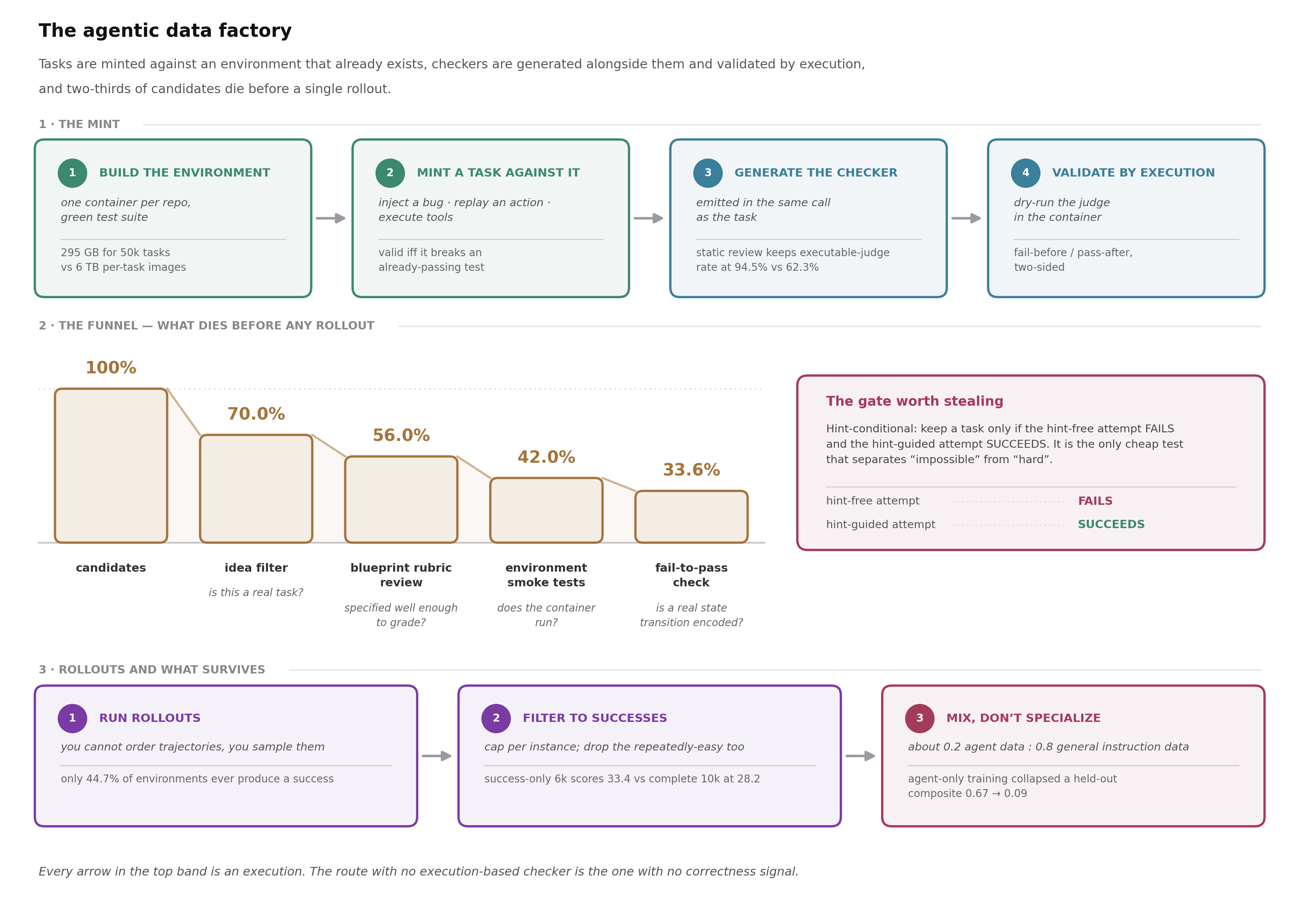 Figure 5. The agentic data factory: tasks minted against an already-built environment, checkers generated alongside them and validated by execution, and two-thirds of candidates discarded before a single rollout.
Environments first, tasks minted against them
Build the environment once and mint tasks against it. SWE-smith builds one Docker image per repository with a mostly-passing test suite, then injects bugs into it; a candidate is valid if and only if it breaks an already-passing test, so execution supplies the task and the grader at once. 128 repositories give 50,137 instances for $1,360 and about 20 hours of human time, most of it verifying install specs an agent wrote (Yang et al., 2025). One image per repository costs 295 GB for 50k tasks; one image per task costs 6 TB for 2,438.
The rest of the field is reverse construction run against a live system. Do something, observe what changed, describe it afterwards, and the task is executable by construction because it was derived from an execution.
| Route | Executed first | Checker comes from | Measured yield or cost |
|---|---|---|---|
| Inject a bug into a green repo (SWE-smith) | apply a diff, run the suite | pre-existing tests the bug breaks | 50.1% of candidates break a test, 2.32¢ each |
| Commit → generated test → issue (R2E-Gym) | run generated fail-to-pass tests | generated or existing tests | 8,135 executable tasks; 4,578 in the 10-repo training subset |
| Blind UI traversal (OS-Genesis) | click, type, scroll; record before/after | nothing executable, a 1–5 model score | 1K trajectories, AndroidWorld 9.82 → 17.41 |
| Execute tools, then derive a query (DIVE) | 6 tool calls × 3 rounds on live APIs | reference answer, two cross-verifiers | 373 validated tools, ~42% keep rate |
| Spec → grounded blueprint → image (CLI-Universe) | research the spec, then build it | a role-separated test agent | 33.6% of candidates survive all gates |
| Proposer emits task and judge (VERIGEN) | dry-run the judge in a container | the generated Python judge | 94.5% executable, $0.93–1.01 per task |
Six routes to an agentic example. The one route with no execution-based checker also has no correctness signal.
Generate the checker in the same call as the task, then validate it by running it. VERIGEN’s proposer emits a task plus an executable judge, a second role reviews that judge statically, and a third dry-runs it in a container to test whether the goal state is reachable and correctly scored. Removing the static reviewer drops the executable-judge rate from 94.5% to 62.3% (Lv et al., 2026). Those judges still agree with expert humans on only 82.5% of a 160-trajectory audit, so “verifiable” here means deterministic rather than correct. Diversity, once the checker problem is solved, is structural rather than lexical: 12k tasks spanning 373 tools beat 48k tasks on a fixed two-tool pool at 4× less data (Chen et al., 2026).
Insight — the checker’s author must not see the solution, and the agent must not see the checker. CLI-Universe isolates its test-writing agent from its solution agent (Hua et al., 2026). The mirror-image mistake is leaking the grader into the prompt: SWE-smith students handed the failing test as the issue text attempt reproduction on 127 of 500 runs instead of 379.
The gates that run before you spend a rollout
Rejection is the design, and it belongs before rollouts because rollouts are where the money goes. CLI-Universe retains 100% → 70.0% → 56.0% → 42.0% → 33.6% of candidates through four gates. Its own ablation drops other parts of the pipeline rather than these gates — asset strategy −6.2, test-case rubrics −3.9, query rubrics −3.4 on Terminal-Bench 2.0 — but the shape of the result is that no single component is load-bearing and all of them together are.
| Gate | Question it answers | Measured effect |
|---|---|---|
| Idea filter | is this a real task? | −30.0 pp, at zero execution cost |
| Blueprint rubric review | is it specified well enough to grade? | −14.0 pp; human accept 72% → 91% |
| Environment smoke tests | does the container actually run? | −14.0 pp |
| Hint-conditional | is it non-trivial and solvable? | keep iff hint-free fails and hint-guided succeeds |
| Fail-to-pass | is a real state transition encoded? | −8.4 pp |
| Learnability band | can the policy learn anything from it? | 38k → 3.2k tasks at 1–5 successes in pass@8 (DIVE) |
| Frontier sampling | is it learnable at this checkpoint? | +5.0 OSWorld points, 63.7 → 68.7 (VERIGEN) |
The hint-conditional gate is the one most worth stealing: it is the only cheap test that separates “impossible” from “hard.”
Difficulty is engineered rather than found. CLI-Universe folds real repository and documentation evidence into each spec and reports the pass rate falling from 68.2% to 54.9% as the point of the exercise. VERIGEN weights sampling by a Gaussian on a moving average of each task’s success rate, centered at 0.5, for a mechanical reason: a GRPO group in which every rollout succeeds or every one fails has zero within-group advantage and wastes the whole group.
Trade-off — difficulty demonstrably pays for RL and may not pay for SFT. SWE-smith’s difficulty rater (75.3% accurate on 1,699 human labels) tracks solvability: expert resolve rates are 58.6%, 41.0%, and 17.0% on easy, medium, and hard subsets. But student pass@1 from difficulty-2, -4, -6, and -8 SFT sets of 500 tasks each is 12.4, 10.8, 13.6, and 12.2, which is flat. CLI-Universe is SFT-only and credits difficulty for its gains, so this is an open disagreement, not a settled rule.
Trajectories are the wrong unit to collect and the right unit to filter
You cannot order trajectories the way you order labels. You run rollouts and keep the survivors. SWE-smith made 17,906 attempts across 8,686 instances for 6,457 resolved runs, then capped each instance at three trajectories to reach 5,016 SFT points. R2E-Gym got 3,321 successes from 2,048 of 4,578 environments, so only 44.7% of its environments ever produced one — the majority yielded nothing (Jain et al., 2025).
Filtering to successes is worth more than the data it deletes. Holding tasks and teacher fixed, CLI-Universe’s success-only 6k set scores 33.4 on Terminal-Bench 2.0 while the complete 10k set scores 28.2, so deleting 40% of the corpus is worth 5.2 points. The dissent comes from GUI work, where OS-Genesis grades each trajectory 1 to 5 and samples in proportion to that score rather than gating on it, beating a binary keep-only-complete labeler (Sun et al., 2024). The plausible resolution is domain, since a failed GUI trajectory still contains correct visual grounding while a wrong patch contains a wrong mapping, but nobody has run the crossed experiment. Failure is not really the variable: SWE-smith caps trajectories per instance because repeatedly solved easy tasks also degrade the model, so what hurts is low information at either extreme. What survives goes into a mixture rather than into a model alone, at roughly 0.2 agent to 0.8 general instruction data, because agent-only training collapses a 7B model’s held-out agent composite from 0.67 to 0.09 (Zeng et al., 2023).
Takeaway. Failure trajectories are bad imitation targets, good verifier training data, and excellent curriculum. ARCO (Tian et al., 2026) pairs a deliberately weak policy teacher with a strong rubric teacher, because a near-perfect teacher leaves no faulty actions for the evaluator to learn to penalize. VERIGEN splits a failed task at the earliest step where the rollout deviated, turning each sub-goal into an easier task with its own verifier, worth 4.1 OSWorld points.
Rubrics, and the two ways they fail
A rubric is what you write when no test exists: criteria with signed weights, a judge returning met or not-met for each, and a normalized weighted sum. It is the only mechanism here that scores what execution cannot see. The uncomfortable baseline is that rubric rewards frequently lose to a binary one. On multi-hop QA with a 4B policy, three published rubric-reward methods score 38.00, 34.80, and 32.20 exact match against 39.40 and 41.00 for plain binary-reward RL, with the weakest of them below the untrained base model’s 34.40 and the next essentially tied with it (Tian et al., 2026).
Saturation is the first failure mode. As the policy improves, more of its samples satisfy every criterion and the reward loses variance. Rewarding a co-trained rubric generator for the standard deviation of its scores across sampled answers buys 15.82 → 20.80 at 4B over externally authored golden rubrics, and out of distribution those golden rubrics cost 15.3 points of instruction-following where co-evolved ones gain 6.2 (Ding et al., 2026). That evidence comes from single-turn medical QA with one run per configuration, so it reaches agents by argument.
Mislocation is the second, and it is the one that bites long-horizon agents. With a fresh rubric per action, the only constraint tying step scores to reality is that they sum to the trajectory outcome, which pins the total and says nothing about the distribution. Final-answer step scores predict success at AUROC 0.82–0.87 while intermediate search-step scores manage 0.58–0.65 against 0.50 chance (Tian et al., 2026): the step signal is most reliable exactly where credit assignment matters least. Granularity is non-monotone, peaking at three criteria per step (42.80 exact match, against 41.00 at one and 40.60 at seven), because nine criteria still cover only about three distinct themes.
What is genuinely unsolved here is mostly measurement. Nobody has published a cost per usable trajectory end to end; the roughly $1 per accepted task above covers synthesis only. Nobody has measured what an imperfect judge costs, since 82.5% judge–human agreement and 68.7% OSWorld success are reported together with no estimate of what the missing 17.5% does to the ceiling (Lv et al., 2026). That is the verifier-robustness problem again, worse here because the judge is per-environment rather than shared. And reward hacking on environment state is asserted more than measured: the most-quoted figure, that outcome-only rewards leave roughly 40% of positively reinforced episodes misrepresenting a constraint, appears in prose with no table, sample size, or task set behind it (Arora et al., 2026). Its proposed defense is cheap enough to adopt anyway: compare entity counts at episode end against setup-time baselines, which catches an agent that reached the goal by manufacturing records.
Open question — nobody has isolated the value of recovery. No ablation here trains on trajectories that fail and then recover, as against trajectories that succeed directly. That matters because verification is what frontier agents are worst at: across four frontier models on Terminal-Bench 2.0, verification failures, meaning a plausible attempt that never correctly checks whether the goal state holds, are 47–60% of all failures, more than execution errors (Hua et al., 2026). The behavior your pipeline most needs to teach is the one your success-only filter is least likely to contain.
Distillation as a data-acquisition strategy
Most treatments of distillation are about losses. That framing hides the decision that actually matters. Distillation is a way of acquiring supervision, and every question people ask about it — forward or reverse KL, off-policy or on-policy, can my student beat the teacher, why did a stronger teacher make things worse — is downstream of two facts: what data you can physically extract from the teacher, and how far apart you and the teacher are. Get those right and the loss function follows almost mechanically.
Let me state the practical question directly, because it is the one I have been asked in interviews and the one the rest of this section answers: I have a small model. Frontier models exist and are much better. What do I do?
What you can take, by access tier
Your access tier determines your objective set. It is not a detail; it is the whole design space.
| Tier | What you can extract | Objectives it unlocks | Objectives that are impossible |
|---|---|---|---|
| White-box, same family | the full next-token distribution on any prefix you choose, including the student’s own bad prefixes; hidden states | token-level forward/reverse KL, JSD, sequence-level reverse KL, on-policy full-vocab KL, hidden-state alignment | — |
| Gray-box | top-k log-probs, or the log-prob of your own sampled tokens | top-k KL with a debias term; sampled-token log-ratio used as a policy-gradient advantage; teacher-ratio reweighting of an RL advantage | exact full-vocabulary KL; anything needing teacher entropy |
| Black-box | completions, traces, critiques, scores, preferences, rubrics | SFT on traces; rationale multi-task learning; teacher-as-judge, teacher-as-rubricator, adversarial discriminator as reward | any token-level divergence; dense correction on the student’s own prefix |
| Teacher-free | your own model under privileged context (ground truth, retrieved documents, a constitution) | reverse KL from the privileged-context self to the unconditioned self | anything requiring capability the model does not have |
Access tiers and the objectives they license. The structural problem: signal density and teacher strength are anti-correlated in practice, because the strongest teachers are API-only.
The cost of each step down that ladder is measurable, and smaller than you would guess. Going from full logits to top-k = 128 costs +0.11 nats of validation loss — but top-k = 128 combined with 30% ground-truth next-token loss costs +0.01 nats, statistically indistinguishable from the full distribution (Busbridge et al., 2025). That is the single most practical number in the distillation literature, because full float32 teacher logits cost about 129 KB per token at a 32k vocabulary, which is roughly 260 petabytes for 2T tokens. Truncation plus a little hard-target loss is what makes offline logit reuse physically possible at all.
Going from gray-box to black-box costs you the direction of correction but not all of the signal. Two anchors, both catalogued in the on-policy distillation survey (Song et al., 2026): a 770M model trained on teacher rationales rather than teacher labels beat a 540B teacher with half the examples; and discrete verbal scores from a black-box teacher — literally asking it to grade 0–9 — bought +12.9% exact match on web QA and +25.7% on math. The survey’s summary is worth keeping: on-policy exploration supplies a substantial fraction of the learning signal by itself, and the teacher’s role is closer to selecting among student trajectories than to correcting individual tokens.
Insight — process data is the moat, and the market behaves accordingly. The value gradient of distillable data runs: final answers < code and tool calls < full agent trajectories < raw reasoning traces. The strongest evidence for that ordering is not an experiment, it is a product decision — frontier reasoning APIs expose a summary of the chain of thought while withholding the trace itself. There is also persistent, unverified community reporting of a gray market in extracting exactly that withheld artifact, which I am not going to source or repeat, but whose existence is itself an observation about where value sits. The defensible technical conclusion: if the process is what matters and the process is what you cannot buy, then the objective you want is the one that generates process locally and asks the teacher only to score it — which is on-policy distillation.
The capacity gap
A better teacher can make a worse student, and there is now a number for where that starts. Student cross-entropy follows a broken power law in teacher cross-entropy (Busbridge et al., 2025), with the break at
L_T / L̃_S = 1.315 (90% CI 1.302–1.327)
where L̃_S is the cross-entropy the same student would have reached under ordinary supervised training with the same parameters and tokens. Three things make this the version worth memorizing. It is a ratio of learning capacities, not of parameter counts — relative size is a special case. The teacher enters the law only through its own cross-entropy, so the teacher’s parameter count and token count drop out as search dimensions entirely and you can select a teacher by its validation loss. And the mechanism is measurable: the KL divergence between teacher and student increases with teacher capability, so past the break the student finds the teacher too hard to model and stops benefiting from its improvements.
Two more results from the same law reset default intuitions. Distillation’s loss is less sensitive to parameters and more sensitive to tokens than supervised training’s — the fitted exponents move from α = 0.408, β = 0.431 to α = 0.321, β = 0.637. Because the compute-optimal parameter share is β/(α+β), that pushes the allocation the other way: the parameter share rises from a Chinchilla-like 0.51 to 0.66, and the token share falls from 0.49 to 0.34. Steeper returns to data mean you exhaust the data axis sooner, so the marginal FLOP goes into width. And distillation cannot beat supervised learning asymptotically. The authors’ two-condition test is crisp enough to quote verbatim in a design review: distillation is more efficient if and only if (i) the student’s compute or token budget is below a student-size-dependent threshold, and (ii) a teacher already exists or will be amortized across more than one student. Otherwise, train the student directly. Even weak-to-strong generalization — a student beating its teacher — turns out to be a finite-data artifact: feed the student enough distillation tokens and it drifts back up to the teacher’s cross-entropy.
The runtime version of the capacity gap is cheaper to measure and applies where the scaling law does not. Measure the initial per-token KL between candidate teacher and student on a held-out set. The calibration comes from a controlled swap: replacing a same-origin 30B teacher with an objectively stronger 235B model, holding everything else fixed, took a normalized capability score from 0.937 to 0.600 under one loss and to −1.190 under another, with training diverging catastrophically at step 18. The measured difference between the two configurations was an initial per-token KL of ~0.19 versus ~0.04 (Ma et al., 2026). Under the policy-gradient loss — the one that degraded rather than diverged — the student’s policy entropy contracted from 0.30 to 0.21 as it received predominantly punitive gradient from the teacher’s low-probability regions; the truncated top-k loss is the one that blew up at step 18. If your KL to the teacher starts high, a better teacher is a worse teacher — and that is a pre-flight check costing one forward pass over a validation set, not a training run.
One caveat I want to flag because it is a genuine open disagreement rather than a resolved question: a well-known study sweeping teachers from 340M to 1.5B into a fixed 125M student found student performance positively correlated with teacher size — no capacity gap at all (Gu et al., 2023). The reconciliation on offer is that forward KL’s mode-covering pressure exacerbates the gap while reverse KL’s mode-seeking behavior partially mitigates it, and the scaling law was fit entirely under forward KL. I would treat the 1.315 threshold as well-established for pre-training-style forward-KL distillation and as a useful prior elsewhere.
A playbook: small model, strong teachers
Here is the decision procedure I would actually follow, with the first matching branch winning.
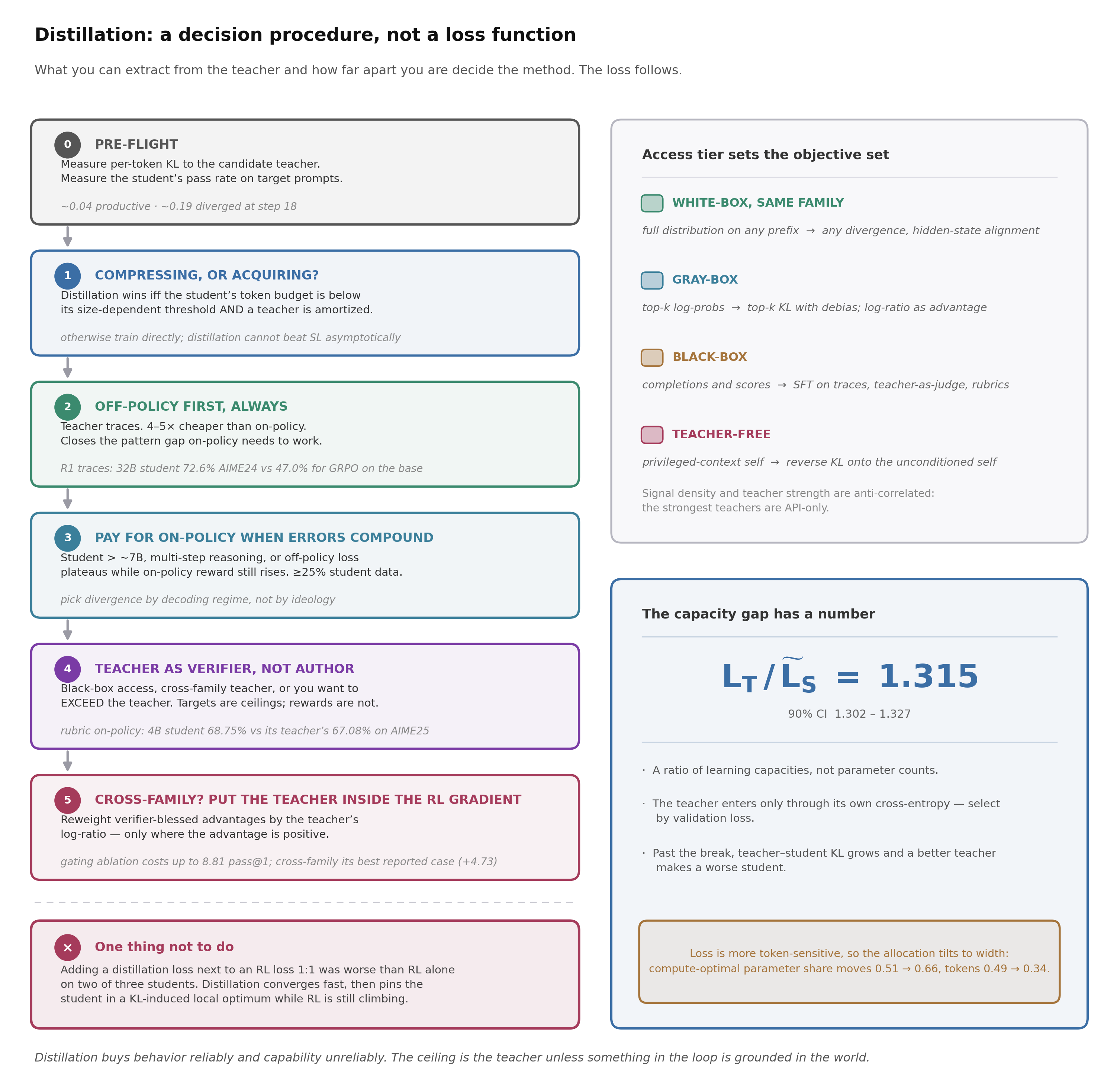 Figure 6. Access tier and capacity gap determine the method; the loss function is the last thing you choose, not the first. Numbers are from the sources cited in this section.
Step 0. Two pre-flight diagnostics. Measure initial per-token KL or top-k overlap between candidate teacher and student (calibration above: ~0.04 productive, ~0.19 failing). Measure your student’s pass rate on the target prompts — if it is near zero, on-policy gradients vanish and you need curriculum pacing or an easier warm-up first.
Step 1. Are you compressing, or acquiring capability? If you are pre-training a smaller model from scratch, apply the two-condition test above literally, and if it fails, just do supervised pre-training. If you are post-training an existing small model, continue.
Step 2. Start off-policy, always. Sequence-level distillation on teacher traces is 4–5× cheaper than on-policy — the survey’s estimate is roughly 300 versus 1,200–1,500 GPU-hours for a 70B→7B setup, which is an order-of-magnitude figure rather than a measured one (Song et al., 2026) — and it closes the pattern gap that on-policy distillation needs in order to work at all. The existence proof that off-policy alone can be sufficient is the R1 distillation series, as reported in that survey: ~800K traces produced a 32B student at 72.6% AIME24 pass@1, against 47.0% for running GRPO directly on the same base. Stay off-policy if the capacity ratio exceeds ~10× and the task admits bounded reasoning depth — factual QA, translation, summarization.
Step 3. Pay for on-policy when the errors compound. Switch when the student is above roughly 7B and exploring off the static-trace manifold, when intermediate errors compound across multi-step reasoning, or when off-policy loss plateaus while held-out reward still improves under on-policy rollouts. Then: turn on at least 25% student-generated data (Agarwal et al., 2023); pick the divergence by decoding regime rather than by ideology (sampled or open-ended generation wants mode-covering, instruction following and single-correct-answer reasoning want mode-seeking); and use full-vocabulary KL if you can afford it, top-k with a debias term if you are shipping the signal over a network, and sampled-token-only if you add variance reduction.
Step 4. Use the teacher as a verifier, not an author, when any of these hold. Access is black-box. Teacher and student are from different families. Or you want to exceed the teacher — which is the decisive case, because distillation targets are ceilings and rewards are not. The existence proof here is striking: a rubric-based on-policy scheme produced a 4B student scoring 68.75% on AIME25 against its own frontier teacher’s 67.08% (Song et al., 2026). The teacher never authored a token of the winning behavior; it only said which of the student’s attempts were good.
Step 5. If you must use a cross-family teacher, put it inside the RL gradient instead of beside it. This is the most useful recent result for the small-model-strong-teacher setting. Rather than matching the teacher’s distribution, use the teacher’s log-probability ratio to reweight the advantage of trajectories the verifier has already blessed, applied only where the advantage is positive. The gating is what makes it work: without it, teacher-preferred tokens on failing trajectories receive a larger penalty, pushing the student away from the teacher. Ablating that single component costs up to 8.81 average pass@1 points (Distilled RL). And the ordering it produces is the opposite of everything else in this section — cross-family becomes the method’s best case in the one pair they report (+4.73 over plain on-policy distillation on a cross-family student, versus +1.16 on a same-family one) — and the proposed reason is that the teacher only ever redistributes a reward-grounded signal and can never drag the student off the verified manifold. Two students is not enough to call it a law. Note the two ordering flips in the same table: in the cross-family setting, plain RL (36.86) beat on-policy distillation (35.27), and naively adding the two losses 1:1 (36.54) still did not beat RL alone.
Step 6. Do not add a distillation loss next to an RL loss and hope. The 1:1 combination was worse than RL alone on two of three students, because distillation converges rapidly and then pins the student in a KL-induced local optimum while RL’s curve is still rising.
There is one more pattern worth knowing even though it needs teachers you probably do not have. If you do control your teachers — for instance if you can afford per-domain RL runs from a shared checkpoint — the strongest result I have seen for combining capabilities is to produce specialists independently and then fuse them in policy space rather than weight space, routing each prompt to its matching teacher during on-policy distillation. That recovers 91–95% of every specialist’s headroom uniformly (normalized score 0.937 against 0.882 for the best baseline and 0.328 for naive weight averaging), and it is iterable: retraining specialists from the fused student pushed the next round’s teachers to 1.030 (Ma et al., 2026). The relevant lesson for everyone else is the precondition — every teacher was an RL descendant of the same SFT checkpoint that initialized the student. Same-origin is doing the work.
Takeaway. Distillation buys behavior reliably and capability unreliably, and the ceiling is the teacher unless something in your loop is grounded in the world. The composite recipe that respects all of that: off-policy traces for the cold start, on-policy correction if the errors compound, the teacher as a scorer rather than an author wherever you want to pass it, and a verifier underneath the whole thing so that the teacher redistributes credit instead of defining the target.
Hygiene for distilled corpora
The failures below are specific to distilled data and mostly invisible to the metric you are optimizing. I have marked which are measured in the literature and which are merely well-motivated, because the distinction gets lost fast in this topic.
Style transfers at nearly 100% and knowledge at nearly 0%, and your judge cannot tell. The foundational result is still the sharpest: fine-tuning open models on a proprietary chat model’s outputs took authoritative tone from 57% to 98% — where the ceiling, measured as one teacher sample against another, is 98% — and list-format matching from 13% to 81% against a ceiling of 83%. Over the same range, Natural Questions accuracy fell from 20 to 15. About 70% of the imitation model’s outputs were rated equal or better than the teacher’s by crowd annotators, and a strong LLM judge showed the same trend (Gudibande et al., 2023). Meanwhile targeted imitation on 6,000 task-local examples took the same benchmark from 20 to 27, against the teacher’s 31. The rule that falls out: never accept a preference win rate as evidence of capability transfer. Pair every judge-based eval with a targeted capability benchmark that your imitation data does not cover, and when they disagree, believe the benchmark.
| Failure | Status | Evidence |
|---|---|---|
| Distribution narrowing / entropy collapse | measured | policy entropy 0.30 → 0.21 under a mismatched teacher (Ma et al., 2026); on-policy distillation lowered one student’s AIME24 pass@16 from 58.33 to 55.00 (Distilled RL) |
| Calibration degradation | measured | forward-KL students end up worse calibrated than the teacher (BoolQ ECE 0.356 teacher → 0.682 student); reverse KL recovers to 0.502 (Gu et al., 2023) |
| Length and format pathologies | measured | raw reverse KL favors short outputs to the point of empty responses (length normalization worth +10.0 ROUGE-L, Gu et al., 2023); the opposite failure, length inflation, appears with reward hints |
| Hacking the teacher’s own likelihood | measured | without teacher-mixed sampling, students learn to emit repeated meaningless strings that have high probability under the teacher — the loss improves as the model gets worse (Gu et al., 2023) |
| Style without substance | measured | see above |
| Bias and safety inheritance | measured in one direction | non-toxicity rises toward the teacher’s level as imitation data grows (Gudibande et al., 2023); the same channel carries the teacher’s biases |
| Contamination laundered through the teacher | plausible, not established | named as a confounder for teachers’ own scores, but I found no paper measuring contamination propagating teacher → student |
| Identity / provenance leakage | plausible, not measured in the literature | no paper in my reading set measures it; the mechanism is a direct consequence of near-complete persona transfer, and anecdotal reports circulate |
Hygiene failures specific to distilled corpora. The last two are the ones people assert most confidently and the ones with the least published evidence.
Two additions to that list from the practical side. The first is the flawed-prefix trap: when the student writes an out-of-distribution prefix, the teacher’s conditional distribution over the continuation is itself poorly calibrated, so you are distilling noise with full confidence. The second is a concrete pipeline item that costs almost nothing: filter or rewrite self-identification strings, vendor names, refusal boilerplate, and system-prompt tics out of teacher traces, and add an identity probe to your eval suite. Identity leakage is the visible end of a general property — distilled corpora carry the teacher’s distributional fingerprints, including its contamination and its safety behavior, whether you wanted them or not.
Insight — inheriting is now much cheaper than learning, which makes it a strategy question. The marginal cost of generating a large corpus of teacher traces has fallen to a rounding error next to a training run, so “inherit or learn” is no longer decided by budget. It is decided by what you want to be true in two years. A pipeline whose every supervision signal comes from a teacher has an implicit roadmap — wait for the next teacher release, add some architecture changes, ship — and its ceiling moves only when someone else’s does. A pipeline with a verifier in it has a ceiling set by the world. The papers say this quantitatively; the industry says it by what it encrypts.
Contamination: your eval set is part of your pipeline
Every stage above separates the artifact you build from the instrument you measure it with. Contamination is where that separation collapses: the eval set is a subset of the training corpus, one distillation hop from it, or something your agent downloads at inference time. That makes it a pipeline problem, not an ethics problem, and it mirrors this post’s question: who guarantees that this example is not in the corpus — and was not in the corpus of the model that generated the corpus?
Where it has been measured cleanly, benchmark overfitting is worth up to 8 accuracy points, and it clusters by model family rather than by model. GSM1k is 1,205 human-written grade-school math problems, matched to GSM8k on resolution-step count and answer magnitude and validated as indistinguishable from it by a human odd-one-out test at 21.83% against 20% chance (Zhang et al., 2024). The drops: Yi-6B-Chat 43.7% → 35.7%, math-shepherd-mistral-7b-rl 82.6% → 75.4%, phi-2 56.6% → 50.4%. Frontier models show nothing — gpt-4o 93.1% → 92.9%, gemini-1.5-flash 79.7% → 83.5%, better on the set that did not exist when it was trained.
Two qualifications. The drop is not the capability: phi-2 loses 6.3 points and still solves more than half of GSM1k, roughly where Llama2-70B lands with 25× the parameters. And the measurement is prompt-dependent — under a second prompt format deepseek-math-7b-rl moves from −3.1 points, which looks clean, to +6.4, which looks badly contaminated.
Detection is a population statistic, not a verdict
The standard membership-inference method is a weak signal cited as if it were proof. Min-K% Prob scores a document by the average log-probability of only its lowest-probability 20% of tokens, on the theory that unseen text contains a few surprising tokens and memorized text does not (Shi et al., 2023). It averages AUC 0.72 across five models on WikiMIA, against 0.67 for plain perplexity. The advertised “7.4% improvement over the best baseline” is relative: +0.05 AUC in absolute terms, which licenses no statement about any single document.
It is weakest where you need it. The same paper’s downstream study reaches 0.86 AUC, but only by continually pretraining LLaMA-7B for a full epoch at lr 1e-4 on a 27M-token corpus with 200 examples from each benchmark inserted; drop the learning rate to 1e-5 and BoolQ detection falls from 0.91 to 0.64. Detection improves with model size, text length, duplicate count and learning rate — the opposite of the case that worries you, a short benchmark item seen once late in training. It needs token log-probabilities, which most frontier APIs no longer expose. As a ratio it is stronger: compared across an unlearned checkpoint and its original, it flagged 188 suspicious book chunks where raw perplexity flagged zero.
Insight — contamination and overfitting are not the same variable. Regressing each model’s per-character log-likelihood on GSM8k against its fresh-set gap gives Spearman ρ = 0.36 (p = 0.03) (Zhang et al., 2024) — real, and a minority of the variance.
math-shepherd-mistral-7b-rlis among the most overfit models yet has one of the lowest likelihoods on GSM8k; the authors’ hypothesis is that its process reward model, trained on synthetic step-level data, leaked correct GSM8k reasoning chains without the problems ever appearing in training. Llemma inverts it: high likelihood, confirmed GSM8k examples in its corpus, minimal overfit.
Decontamination is not a preprocessing step you finish. n-gram and hash matching catch verbatim copies and mirrored dataset dumps and nothing else; embedding similarity catches paraphrase and, with a multilingual encoder, translation, at the price of a recall/precision trade-off that “may result in excessive data removal” (Al-Lawati et al., 2026). No threshold in the chain is justified against a downstream outcome; Min-K%’s k = 20 came from one validation sweep and was then reused everywhere. And filters run “at a fixed point in time” and miss “indirect leakage through continual pretraining, model distillation, or synthetic data generation from contaminated models.” Contamination is a property of a dataset at a moment in a pipeline, not of the dataset.
The channels a corpus filter cannot see
| Channel | What can detect it | Evidence status |
|---|---|---|
| A contaminated teacher writes your SFT data | fresh parallel benchmark only | hypothesized; propagation is unmeasured |
| Reward models and RL prompt sets of benchmark-style problems | fresh parallel set, read per family | one case study; named by GSM1k |
| Synthetic data seeded from the eval distribution | in- vs out-of-distribution divergence | asserted by the Arena audit, not measured |
| Deployment-log recycling | in- vs out-of-distribution divergence | directly measured |
| Eval-time retrieval into clean weights | trajectory audit: URL regex, longest common substring, strict judge | directly measured |
Only the bottom two rest on direct measurement; the top row is the one nearly every 2026 pipeline now has.
Deployment-log recycling is the best-measured of these, and it looks like ordinary product work. Fine-tune one 7B base three times, varying only the share of Chatbot Arena data across 0% / 30% / 70%: the ArenaHard win rate against Llama-3.1-8B-Instruct goes 23.5% → 42.7% → 49.9%, a 112% relative gain, while MMLU goes 66.5% → 64.4% → 65.9% (Singh et al., 2025). No item leaked; the score stopped measuring capability, and the divergence between the two curves is the only tell. The same audit finds 7.3% of December 2024 Arena prompts recurring verbatim in January 2025, and notes you need not train on the logs at all: they also work for seeding synthetic data near the distribution.
Retrieval turns a clean model into a contaminated evaluation. On the first 100 MedQA questions, 60% of Gemini Deep Research’s trajectories visited a page containing both the question and its answer, though search moved its accuracy only from 97% to 99% (Wang et al., 2026). On MedQA, accuracy at the turn before explicit answer leakage is 7.69% and at the turn after is 89.74% (n = 39), a Cox hazard ratio of 4.21. Two caveats: URL-level metadata hits carry hazard ratios below 1 on five of six benchmarks, so coarse detection misleads, and the “up to 4%” inflation headline is never derived — the closest quantity, a 4.05-point gap on HLE-149, is −1.50 on MedQA and −2.90 on MedMCQA. All six benchmarks are clinical, so generality is asserted rather than shown. The portable finding is provenance: one agent with a curated PubMed index leaks 0% on MedQA and 65 of 100 sampled PubMedQA questions, because PubMedQA is built from PubMed.
Eval integrity is a systems property
No filter fixes this; the failures live in different parts of the system.
Takeaway. Four instruments. Report one clearly out-of-distribution eval beside every headline number and read the divergence, not either number. Attach an attempt count to every score: two byte-identical Aya-Vision-8B checkpoints submitted to Chatbot Arena scored 1069 and 1052 with four models ranked between them (Singh et al., 2025). If your system retrieves, run every eval search-on and search-off and publish the answer-leakage rate beside the accuracy. And hold back a canary split of vetted items, which is how GSM1k detects leakage through the vendor APIs it needed to score closed models.
Private held-out sets buy clean measurement at the cost of independent verification, and need weight sharing or API access that re-exposes the items. Dynamic regeneration resists item-level leakage but destroys longitudinal comparability.
Open question — can a benchmark be published in a form you cannot train on? The most interesting proposal exploits the training/inference asymmetry in Transformers: release each question’s KV cache and penultimate-layer hidden state, keep only the answer in plaintext, and the item is usable for inference but useless for a gradient step (Al-Lawati et al., 2026). It is a position paper with no experiments, its own cited literature says KV-cache inversion attacks work on multi-head attention and are merely “much less effective” on grouped-query attention, and whoever holds the anchor model still sees the plaintext. Two adjacent things are also unmeasured: contamination propagating from a teacher into a student, and whether an LLM judge was trained on the eval it scores.
The data platform
If the argument of this post is right — that the unit of data changes from text to software as you climb the stack — then the thing a serious lab builds is not a dataset but a platform. Interviewers ask about this obliquely (“how would you set this up?”) and it is worth having a concrete answer, so here is the component list implied by everything above.
A provenance and lineage service. Every training example needs to carry where it came from, which generator and prompt produced it, which certifier passed it, and which runs consumed it. This is not bureaucracy: provenance is what lets you answer “is this corpus real or synthetic, and does the real part stay in?” — the question that decides whether accumulation protects you from collapse. It is also the only way to retract data after you discover a contaminated source, and the cheapest capacity intervention available, since prepending a provenance token to documents recovered most of a 20× capacity loss from corpus dilution (Allen-Zhu and Li, 2024).
A decontamination service, not a decontamination script. Prompt-side n-gram matching, run against every eval you report, on every corpus you add, including synthetic corpora and RL prompt sets. It belongs in the platform rather than in each project because the published overlap rates are alarming enough that you will not remember to run it manually.
A scorer registry. Quality classifiers are the highest-leverage knob in pre-training and the most dangerous one in mid-training, because they are length-biased and will silently delete your long-context and agent-trajectory data. Register each scorer with the source distribution it was calibrated on, its length-response curve, and the threshold in use — and always report random selection with source preservation as a baseline, since it beats most published filters.
A verifier registry with adversarial suites attached. Every checker is a piece of software with a version, a measured precision and recall on your data, and a suite of adversarial patterns it must resist. The non-negotiable lesson from the ladder section is that static accuracy does not predict RL outcome, so the artifact you version is the verifier plus its attack suite, and the suite has to be regenerated as policies get stronger.
An oracle channel. At every checkpoint, sample ~1,000 training prompts, regenerate, and score them with a strong external model. Plot training reward and oracle reward on the same axes. Divergence between those two curves is the most reliable reward-hacking alarm I know of, and unlike a held-out eval it costs one generation pass per checkpoint.
An environment registry. Container images, seeds, task specifications, rubrics, and a two-sided validation record showing the checker fails on the unfixed instance and passes on the fixed one. This is the part that is unambiguously software engineering, and the part where headcount goes at the top of the stack.
Private, rotating, and freshly collected evals. Whatever you publish, keep a held-out set that never leaves the building, rotate a fraction of it on a schedule, and maintain a non-regression suite that runs on every checkpoint. The reason is in the contamination section, and the incentive analysis behind it is simple: contamination is not only an accident of web crawling, it is what an organization drifts toward when its objective function collapses to a score.
A decision guide
Compressed answers to the questions this post exists to answer. Each one is defensible from evidence above; none is a substitute for measuring on your own stack.
| Question | Short answer |
|---|---|
| Synthetic or real? | Wrong axis. Ask who certifies correctness. The most reliable “synthetic data” wins are synthetic labels over real text, not synthetic text. |
| Should I fear model collapse? | Only if you replace data. Under accumulation the error is bounded by a constant; under replacement it diverges. Never replace, always accumulate — and note every published collapse experiment is ≤126M parameters. |
| Is my quality filter good? | Compare it to random selection with source preservation, and check its length-response curve. Human agreement is a poor predictor of downstream gain. |
| How much should I deduplicate? | Per-snapshot, not globally. Aggressive global dedup preferentially keeps ads and keyword spam. |
| What LR for continual pre-training? | ~5e-5 for an 8B-class model on tens of billions of tokens. Do not tune warmup length; do estimate the checkpoint’s equivalent pre-training compute first. |
| What replay ratio? | By shift magnitude, not budget: 1–5% for a same-language refresh, ~25% for a new language or domain, 30–60% in production runs. |
| Will my model learn facts from my documents? | Not from raw documents. Rewrite each fact into ≥5 surface forms with varied order, or mix QA-format data into pre-training. Augmenting a subset teaches the storage convention and transfers. |
| Fine-tune or retrieve? | Retrieve if you can. Synthetic continued pre-training bought ~80% of retrieval’s gain with no test-time corpus access, and they compose. |
| How do I validate a long-context recipe? | Not on perplexity and not on needle-in-a-haystack. Evaluate after SFT, on retrieval and re-ranking and ICL, and check short-context regressions against the base model. |
| How much SFT data? | Undefined until you name the base model and the eval breadth. A behavior costs 6–30 examples; a 12-skill average was still improving at ~940K. |
| Which SFT selection signal? | Any relative one (rank evolved variants, measure solve rate, embedding distance to selected). Absolute ones — perplexity, instruction length, isolated 1–10 judgments — lose to random. |
| What is an RL example? | A task plus a checker. Keep prompts with reward variance; exclude never-solved prompts, which are worse than absent. |
| Is my RL gain real? | Run format-only reward, random reward, a non-Qwen base, and a post-cutoff benchmark. Random rewards reproduced 73% of the ground-truth gain on Qwen2.5-Math-7B (Shao et al., 2025). |
| Rule-based or model verifier? | Rule first, model verifier on the residual. Choose by adversarial robustness, never by held-out accuracy; discriminative judges resisted attack 20–200× better than generative ones, depending on the attack. |
| Distill or RL? | Distill to reach the teacher, RL to pass it. If you need cross-family transfer, put the teacher inside the RL advantage rather than beside it. |
| Which teacher? | The one closest to you in initial per-token KL, not the strongest. ~0.04 works; ~0.19 degraded and then diverged. Select by cross-entropy, not parameter count. |
| Off-policy or on-policy distillation? | Off-policy first, always — 4–5× cheaper and it closes the pattern gap. Pay for on-policy when intermediate errors compound. |
| Did my distillation work? | Check pass@k, calibration, and a capability benchmark your imitation data does not cover. Being rated equal or better than the teacher on 70% of prompts is compatible with losing 5 points of factual accuracy. |
Open problems
The gaps below are the ones I could not resolve from the literature, stated precisely enough to be worth working on.
Nobody has measured the interaction between replay ratio and knowledge augmentation. The augmentation papers fix replay at 10% and never sweep it; the replay papers sweep it and never augment; two major mid-training studies report no replay ratio at all because they fold general web data into the mixture instead. If there is a unified continual-pre-training knob set, this is the missing cell.
Model collapse has never been tested at frontier scale. Every accumulation-versus-replacement experiment in print is at 126M parameters or below, and the accumulation bound is π²/6 ≈ 1.645× the single-iteration error (Gerstgrasser et al., 2024) — a real 64% penalty, not zero. Whether that constant holds, grows, or shrinks with scale is unknown and is a load-bearing assumption behind the entire synthetic-data strategy.
Proxy-based mixture optimization has no method that survives its own assumptions. Rank invariance fails for at least three independent reasons — a repetition confound, genuine movement of the optimum with scale, and sensitivity to domain granularity — and the method that made the field standard loses to uniform sampling when domains are defined semantically instead of by provenance. There is no accepted replacement.
There is no verifier benchmark that predicts RL outcomes. The one clean experiment on this point is a negative result: a verifier improved on static recall and precision produced the worst RL run in its paper. Until someone builds an evaluation whose ranking correlates with downstream RL performance, verifier selection remains an empirical, per-project exercise.
Contamination propagating from teacher to student is unmeasured. It is widely asserted and mechanistically obvious — distilled traces carry the teacher’s exposure — but I found no paper that measures the effect size. The same goes for identity and provenance leakage, which is a direct prediction of near-complete persona transfer and yet has no published measurement.
Conditioned diversity and sampled diversity have never been combined. Persona conditioning moves the generator’s mode many times; distribution-level prompting flattens the distribution being sampled. Both work. As far as I can tell nobody has run them together, and the second is nearly free.
The capacity gap under reverse KL and on-policy sampling is unresolved. The 1.315 threshold was fit entirely under forward, off-policy KL, and at least one careful study finds no gap at all under reverse KL (Gu et al., 2023). Since almost all practical post-training distillation is reverse-KL and on-policy, this is the version of the law people actually need and the version nobody has.
Data attribution is missing at every stage. Not a single result in this post can tell you which training examples produced which capability. Every selection method in the literature is a proxy for an attribution question we cannot yet answer, which is why so many of them lose to random selection.
Appendix: interview questions
I wrote this post partly to stop improvising answers to these. The pattern in every good answer is the same three moves: name the stage, name who certifies correctness there, and give a number with its baseline. What follows is the compressed version; the sections above are the working.
Framing
“Synthetic data or real data?” Reject the axis, then rebuild it. The question that predicts behavior is who supplies the correctness signal — humans, a teacher, or the world — and every recipe is a portfolio over those three that rotates as you climb the stack. Then give the load-bearing observation: the largest reliable synthetic-data wins are synthetic labels over real text, not synthetic text. One corpus reached 33.6% MMLU at 38B tokens where the next-best needed ~300B, and the mechanism was a 70B model scoring 460k pages for educational value, distilled into a cheap classifier and applied to 15T tokens for ~6,000 H100-hours.
“What is the actual bottleneck in training data today?” Verification, and it inverts as you climb. At the bottom you have 10⁹–10¹⁰ documents and zero verification cost per document; at the top you have 10²–10⁴ tasks each of which may need a container and a validated checker. Per-example verification cost rises by five or six orders of magnitude while example count falls by the same, which is why “get more data” is right at the bottom and almost always wrong at the top.
“How do you think about data quality?” Quality is not a property of a document, it is a relation between a document and a task. The evidence: a filter that agreed with human annotators at ~82% ROC-AUC produced worse models than a plain bigram classifier, and the correlation between annotator agreement and downstream score had R² < 0.3. Choosing the positive-class reference corpus mattered more than choosing the classifier — instruction data plus a plain-explanations subreddit beat a Wikipedia-and-books reference set by 3.5 points.
Pre-training
“Is pre-training data a solved problem?” No, and three received beliefs were overturned recently. Deduplication is not monotonically good — global cross-snapshot dedup preferentially keeps ads and keyword spam, and on one crawl the 31B tokens that survived it trained a worse model than the 171B tokens it had thrown away. Filtering beats architecture as a lever, and it is a reference-corpus decision. And the unit of selection can be smaller than the document: in a filtered math corpus, 51% of tokens are already learned, 26% are where learning happens, 11% are irreducibly hard, and 12% get worse during training; masking loss to the top ~60% by excess loss let a 7B model match a 500B-token specialist using 15B tokens.
“Are we running out of data?” The careful forecast: ~510T tokens indexed, ~100T after quality adjustment, ~320T after allowing repetition, demand growing ~2.4×/year, median crossing around 2028. Then add the repetition result: up to 4 epochs is nearly free, gains continue to ~16, and by 40 epochs repeating is worthless — with the important corollary that when you are data-constrained you should buy epochs before parameters, because repeated tokens decay in value more slowly than excess parameters do. Then undercut yourself honestly: the optimal number of passes is model-size dependent, ranging from ~24 at 30M to ~5 at 757M in one 2026 study, so “four epochs” is a number from one scale, not a law.
“Doesn’t training on synthetic data cause model collapse?” Only under a protocol nobody uses. The original result replaces the previous generation’s data each round; under accumulation — which is what actually happens on the web — test error is provably bounded by a constant independent of the number of iterations, versus linear divergence under replacement, and cross-entropy stays flat over five iterations empirically. The operational rule is never replace, always accumulate. The honest caveats: the accumulation bound is still π²/6 ≈ 1.645× the single-iteration error, and every experiment in print is at ≤126M parameters.
Mid-training and continual pre-training
“Design a mid-training corpus for domain X.” Answer in the knob set, not in vibes: most-converged or non-decayed checkpoint; ~1% warmup, peak LR ~5e-5, cosine to 0.1×; replay set by shift magnitude (1–5% weak, ~25% strong); a mixed corpus, never domain-sequential; ~1% instruction data so the policy does not degenerate later; every domain you will ever want, because you cannot add one at RL time; ~15–27B tokens at 16K context; and a separate long-context repair stage. Then say how you will evaluate it, which is the part that distinguishes a good answer: after SFT, on things you did not train, and — if RL follows — by post-RL performance rather than by the checkpoint’s own scores.
“Why does continual pre-training cause forgetting?” Partly it does not. Re-warming and re-decaying on the exact same data the model was pretrained on still raises validation loss by +0.1 to +0.2 nats, against +0.35 to +0.45 with a real distribution shift. So a meaningful fraction of what gets called forgetting is the optimizer, which is why infinite learning-rate schedules and resuming from non-decayed checkpoints exist. Then quantify the replay fix: 1% replay recovered 0.18 of a 0.27-nat regression at zero cost on the new data.
“How do you inject proprietary knowledge into a model?” Lead with the failure. A model can memorize a corpus token by token and still answer only 9.7% of questions about held-out entities in it, against a 2.7% majority baseline, and no fine-tuning configuration fixes it — one 682M-parameter run hit 99.0% on the QA pairs it was tuned on and 4.4% on the held-out ones after 1,350 passes over the corpus. The reason is placement, not capacity: the fact sits diffusely across the document rather than on the entity’s name, which is all a question supplies. Then the fix and its shape: five distinct rewrites plus sentence permutation reach 96.6%; five rewrites in fixed order reach only 41%; permutation alone hurts. Then the two multipliers: augmenting a disjoint subset teaches the storage convention and lifts untouched documents from 4.4% to 86.8%, and mixing QA-format data into pre-training reaches 86.6% with no augmentation at all. Then the production version: relation-graph expansion inflated 1.3M real tokens to 455M synthetic and moved closed-book accuracy 39.49 → 56.22, which is ~80% of what retrieval bought, while continued pre-training on the raw 1.3M tokens scored 38.15 — below the base model.
“How much data do you need for long context?” 500M tokens unlocks most of it, 5B is the peak, 10B starts to regress because the model overfits its training range. But spend the answer on methodology instead: two mixtures differing by ≤0.01 nats at every length differ dramatically on retrieval, perplexity improves as long-task performance falls, and a model scoring 100 on needle-in-a-haystack scored 23.1 on re-ranking. Also: 60% long / 40% short beats 100% long even for long tasks, train at 512K to be good at 64K, and curate the short stream because it is what keeps your math scores alive.
“Why does R1-Zero-style RL work on some base models and not others?” Because RL amplifies what the base can already sample, and the fix is mid-training. Under GRPO one family’s base ran its length to the cap and degenerated into repeated “Solution” tokens; 200B tokens of math mid-training plus a 20B decay branch took MATH500 from 10.0 (base + RL) to 65.2. What was installed was a parseable format, ~1% instruction-following, and a corpus good enough to sample correct solutions from. The weight-level evidence is the closer: mid-training moves >90% of parameters, RL moves ~5% — a 580× smaller update that leaves representational geometry at CKA > 0.998 — and changing the RL mixture moved a six-benchmark average by −0.21 while changing the mid-training mixture moved it +5.60 and +17.34 on GPQA-Diamond.
SFT
“How much SFT data do you need?” The question is underspecified, and saying so with a number is the answer. Identical 800 curated examples gave 9.2% and 63.3% AIME24 on Qwen1.5-32B-Chat and Qwen2.5-32B-Instruct — a 54.1-point swing from the base model, larger than any data intervention I found. Eval breadth explains the rest: a single chat metric plateaus by ~2K examples; a 12-skill average was still improving at 939,344. And the unit is a behavior, not an example: 30 examples installed multi-turn dialogue, 6 installed structured output.
“How would you select 10K examples from a 1M pool?” Correctness gate first, because wrong data has negative value — one 100K uncurated reasoning corpus scored 17.6 points below the un-fine-tuned base. Then prompt diversity, because it sets the ceiling and because the largest single ablation in the most thorough open recipe was removing diversity-injecting persona data (−19.2 IFEval). Then response quality. Then quantity. For the mechanics, insist on relative signals: rank evolved variants in one prompt rather than scoring examples in isolation, or measure a solve rate. Absolute signals lose to random — perplexity scored 4.06 and 1.89 where random scored 5.84 and 4.93.
“What is the cheapest big win in a synthesis pipeline?” A prompt rewrite. Synthetic competition-math data from two frontier generators with an ordinary prompt drove a three-benchmark average to 30.6, below the 32.8 you get by not fine-tuning at all. Ask the same models for “five responses with their probabilities” and it goes to 36.1, or 37.5 for the multi-turn variant. The mechanism is that preference annotators systematically prefer higher-base-log-probability text independent of quality, with a fitted coefficient of 0.57–0.65 at p < 10⁻¹⁴, so under a reward modeled that way, alignment sharpens the model onto its base mode wherever true quality is flat across candidates.
RL and agentic RL
“What does an RL dataset consist of?” Tasks and checkers, not answers. Keep prompts with reward variance, because a group-normalized advantage produces no gradient at all when every rollout in a group scores the same. Exclude never-solved prompts: training on an unsolvable problem drove one benchmark to 45.0, below the 65.6 from a format-only reward. And distinguish the three reasons a prompt is never solved — too hard, mislabeled, unverifiable — because zero-pass buckets are enriched in broken tasks.
“How do you know your reward is not being hacked?” Two instruments and one habit. An adversarial pattern suite, because across 13 attack patterns discriminative verifiers suffered 0.1–0.4% attack success while generative chain-of-thought verifiers ranged 7.7–23.7%, with one cell at 77.9%. An oracle channel: re-score ~1,000 sampled training prompts with a strong external model at every checkpoint and plot training reward against oracle reward on the same axes; divergence is the most reliable alarm of the three. And the habit of never selecting a verifier by held-out accuracy — the one paper that tried improving a verifier’s static recall from 0.49 to 0.62 produced its worst RL run, because the policy learned to emit a single {.
“Is RLVR teaching the model or eliciting what is already there?” It depends on the (model, domain) pair, and that is measurable. On one math-specialized 7B base, random rewards bought +21.4 points against +29.1 for ground truth — 73% of the gain from a coin flip — via a GRPO clipping bias that ratchets up already-likely tokens. On a base without that prior, ground truth gained +15.5 and every weak alternative lost points. So run four controls: format-only reward, random reward, a non-Qwen base, and a post-cutoff benchmark. If format reward captures most of your gain you are eliciting, the reward content is nearly fungible, and your verifier investment is wasted.
“How noisy can your labels be?” More than you would think in one direction and much less in the other. Unbiased noise degrades: 60% randomly wrong labels cost ~1.3 average points. Biased noise steers: on a single training example, a wrong-but-plausible answer scored 57.0 against 64.4 for a wrong-and-unreachable one and ~74 for the correct one. The dangerous mislabel is the plausible one, and a rule verifier’s false negatives are biased by construction — they concentrate on the most novel correct answers and get worse as your policy improves.
Distillation
“I have a small model and frontier models exist. What do you do?” Answer in the order of the decision tree. Check the initial per-token KL to each candidate teacher first (~0.04 productive, ~0.19 degrading), then your student’s pass rate on the target tasks. Cold-start off-policy on teacher traces, which is 4–5× cheaper and closes the pattern gap; ~800K traces produced a 32B student at 72.6% AIME24 against 47.0% for RL on the same base. Move to on-policy only when intermediate errors compound. If your teacher is a different family or you need to pass it, stop matching it: use it to score, rubricate, or reweight advantages on verified-positive trajectories.
“Can a student beat its teacher?” Yes, but only through a channel that is not imitation. Distillation targets are ceilings; rewards are not. One rubric-based on-policy scheme produced a 4B student at 68.75% on AIME25 against its frontier teacher’s 67.08% — the teacher authored none of the winning behavior, it only judged. Asymptotically, distillation cannot beat supervised learning, and even weak-to-strong generalization is a finite-data artifact that disappears with enough tokens.
“Why would a stronger teacher make my student worse?” The capacity gap, and there is a number: the break in the fitted law sits at a teacher-to-student cross-entropy ratio of 1.315, and it is a gap in learning capacity rather than in parameter count. The runtime version is a controlled swap where replacing a same-origin teacher with a much stronger one from another family took a normalized score from 0.937 to 0.600, and to −1.190 under a truncated loss with divergence at step 18 — with initial per-token KL of ~0.19 versus ~0.04. Under the policy-gradient loss the student’s entropy contracted from 0.30 to 0.21 as it absorbed punitive gradient from the teacher’s low-probability regions; the truncated loss is the one that diverged.
“Forward KL or reverse KL?” It is a function of what you measure, and saying so is the answer. On pre-training cross-entropy, forward KL beat reverse by 0.28 nats — 2.42 against 2.70 — at half the cost (Busbridge et al., 2025). On free-run instruction following, forward KL left the student worse calibrated than the teacher (ECE 0.682 against the teacher’s 0.356) with growing exposure bias. Forward KL optimizes the metric it is trained on; reverse KL optimizes what the model emits at temperature — and reverse KL trades pass@k for pass@1, which matters if RL comes next.
“What are the risks of training on distilled data?” Style transfers at ~100% and knowledge at ~0%, and your judge cannot tell: authoritative tone went 57% → 98% against a 98% ceiling while factual accuracy fell from 20 to 15, with ~70% of outputs rated equal or better than the teacher. Then list the measured hygiene failures — entropy collapse, calibration degradation, length pathologies, hacking the teacher’s own likelihood — and be honest that the two failures people assert most confidently, contamination laundered through a teacher and identity leakage, have the least published evidence. Then give the cheap mitigations: strip self-identification and refusal boilerplate, add an identity probe to the eval suite, and pair every judge-based eval with a capability benchmark your imitation data does not cover.
Evaluation and contamination
“How do you know your benchmark number is real?” Treat your eval set as part of the pipeline. Prompt-side n-gram decontamination against every eval on every corpus including synthetic ones and RL prompt sets; a private held-out set that never leaves the building; a rotating fraction; a non-regression suite on every checkpoint; and at least one benchmark collected after your data cutoff. The reason to be systematic rather than diligent is the published overlap rates: Tülu 3’s own audit of widely used instruction sets found Evol CodeAlpaca overlapping 70.7% of HumanEval and LMSys-Chat-1M overlapping 46.5% of AlpacaEval, and they excluded four datasets outright rather than clean them (Lambert et al., 2024). The same team tried embedding-based detection and abandoned it, because it cannot distinguish distributional similarity from actual paraphrase, while n-grams still catch the case that matters most: a math problem where only the numbers changed.
How to cite
Zhang, Jiaxin. (Jul 2026). Where Training Data Comes From: Synthesis, Verification, and Distillation Across the Training Stack. Jiaxin Zhang’s Blog. https://jxzhangjhu.github.io/blog/2026/where-training-data-comes-from/
@article{zhang2026trainingdata,
  title   = "Where Training Data Comes From: Synthesis, Verification, and Distillation Across the Training Stack",
  author  = "Zhang, Jiaxin",
  journal = "Jiaxin Zhang's Blog",
  year    = "2026",
  month   = "Jul",
  url     = "https://jxzhangjhu.github.io/blog/2026/where-training-data-comes-from/"
}
References
[1] Rishabh Agarwal, et al. “On-Policy Distillation of Language Models: Learning from Self-Generated Mistakes.” arXiv:2306.13649, 2023.
[2] Ali Al-Lawati, et al. “LLM Benchmark Datasets Should Be Contamination-Resistant.” arXiv:2605.19999, 2026.
[3] Zeyuan Allen-Zhu, et al. “Physics of Language Models: Part 3.1, Knowledge Storage and Extraction.” arXiv:2309.14316, 2023.
[4] Zeyuan Allen-Zhu, et al. “Physics of Language Models: Part 3.3, Knowledge Capacity Scaling Laws.” arXiv:2404.05405, 2024.
[5] Akshay Arora, et al. “Beyond Static Evaluation: Building Simulation Environments for Scalable Agentic Reinforcement Learning.” arXiv:2607.05773, 2026.
[6] Dan Busbridge, et al. “Distillation Scaling Laws.” arXiv:2502.08606, 2025.
[7] Aili Chen, et al. “DIVE: Scaling Diversity in Agentic Task Synthesis for Generalizable Tool Use.” arXiv:2603.11076, 2026.
[8] Rui Dai, et al. “Explaining Data Mixing Scaling Laws.” arXiv:2606.08167, 2026.
[9] Hongxin Ding, et al. “EvoRubrics: Dynamic Rubrics as Rewards via Adversarial Co-Evolution for LLM Reinforcement Learning.” arXiv:2606.23038, 2026.
[10] Yao Fu, et al. “Data Engineering for Scaling Language Models to 128K Context.” arXiv:2402.10171, 2024.
[11] Tianyu Gao, et al. “How to Train Long-Context Language Models (Effectively).” arXiv:2410.02660, 2024.
[12] Tao Ge, et al. “Scaling Synthetic Data Creation with 1,000,000,000 Personas.” arXiv:2406.20094, 2024.
[13] Matthias Gerstgrasser, et al. “Is Model Collapse Inevitable? Breaking the Curse of Recursion by Accumulating Real and Synthetic Data.” arXiv:2404.01413, 2024.
[14] Yuxian Gu, et al. “MiniLLM: On-Policy Distillation of Large Language Models.” arXiv:2306.08543, 2023.
[15] Arnav Gudibande, et al. “The False Promise of Imitating Proprietary LLMs.” arXiv:2305.15717, 2023.
[16] Suriya Gunasekar, et al. “Textbooks Are All You Need.” arXiv:2306.11644, 2023.
[17] Kshitij Gupta, et al. “Continual Pre-Training of Large Language Models: How to (re)warm your model?.” arXiv:2308.04014, 2023.
[18] Zhanbo Hua, et al. “CLI-Universe: Towards Verifiable Task Synthesis Engine for Terminal Agents.” arXiv:2606.22883, 2026.
[19] Yuzhen Huang, et al. “From Accuracy to Robustness: A Study of Rule- and Model-Based Verifiers in Mathematical Reasoning.” arXiv:2505.22203, 2025.
[20] Adam Ibrahim, et al. “Simple and Scalable Strategies to Continually Pre-train Large Language Models.” arXiv:2403.08763, 2024.
[21] Naman Jain, et al. “R2E-Gym: Procedural Environments and Hybrid Verifiers for Scaling Open-Weights SWE Agents.” arXiv:2504.07164, 2025.
[22] Carlos E. Jimenez, et al. “SWE-bench: Can Language Models Resolve Real-World GitHub Issues?.” arXiv:2310.06770, 2023.
[23] Nathan Lambert, et al. “Tülu 3: Pushing Frontiers in Open Language Model Post-Training.” arXiv:2411.15124, 2024.
[24] Xian Li, et al. “Self-Alignment with Instruction Backtranslation.” arXiv:2308.06259, 2023.
[25] Jeffrey Li, et al. “DataComp-LM: In search of the next generation of training sets for language models.” arXiv:2406.11794, 2024.
[26] Xuefeng Li, et al. “LIMR: Less is More for RL Scaling.” arXiv:2502.11886, 2025.
[27] Zhenghao Lin, et al. “Rho-1: Not All Tokens Are What You Need.” arXiv:2404.07965, 2024.
[28] Wei Liu, et al. “What Makes Good Data for Alignment? A Comprehensive Study of Automatic Data Selection in Instruction Tuning.” arXiv:2312.15685, 2023.
[29] Bowen Lv, et al. “ScaleCUA: Scaling Computer Use Agents with Verifiable Task Synthesis and Efficient Online RL.” arXiv:2607.11185, 2026.
[30] Wenhan Ma, et al. “MOPD: Multi-Teacher On-Policy Distillation for Capability Integration in LLM Post-Training.” arXiv:2606.30406, 2026.
[31] Pratyush Maini, et al. “Rephrasing the Web: A Recipe for Compute and Data-Efficient Language Modeling.” arXiv:2401.16380, 2024.
[32] Arindam Mitra, et al. “AgentInstruct: Toward Generative Teaching with Agentic Flows.” arXiv:2407.03502, 2024.
[33] Niklas Muennighoff, et al. “Scaling Data-Constrained Language Models.” arXiv:2305.16264, 2023.
[34] Guilherme Penedo, et al. “The FineWeb Datasets: Decanting the Web for the Finest Text Data at Scale.” arXiv:2406.17557, 2024.
[35] Ziyun Qiao, et al. “HERMES: A Multi-Granularity Labeling Substrate for Pre-training Data Mixtures.” arXiv:2607.02266, 2026.
[36] Qwen Team “The Verification Horizon: No Silver Bullet for Coding Agent Rewards.” arXiv:2606.26300, 2026.
[37] Aswin RRV, et al. “Mid-Training with Self-Generated Data Improves Reinforcement Learning in Language Models.” arXiv:2605.08472, 2026.
[38] Bharat Runwal, et al. “PRISM: Demystifying Retention and Interaction in Mid-Training.” arXiv:2603.17074, 2026.
[39] Rulin Shao, et al. “Spurious Rewards: Rethinking Training Signals in RLVR.” arXiv:2506.10947, 2025.
[40] Weijia Shi, et al. “Detecting Pretraining Data from Large Language Models.” arXiv:2310.16789, 2023.
[41] Ilia Shumailov, et al. “The Curse of Recursion: Training on Generated Data Makes Models Forget.” arXiv:2305.17493, 2023.
[42] Shivalika Singh, et al. “The Leaderboard Illusion.” arXiv:2504.20879, 2025.
[43] Mingyang Song, et al. “A Survey of On-Policy Distillation for Large Language Models.” arXiv:2604.00626, 2026.
[44] Qiushi Sun, et al. “OS-Genesis: Automating GUI Agent Trajectory Construction via Reverse Task Synthesis.” arXiv:2412.19723, 2024.
[45] Zihang Tian, et al. “ARCO: Adaptive Rubrics with Co-Evolution for Multi-Step LLM-Based Agents.” arXiv:2606.21262, 2026.
[46] Pablo Villalobos, et al. “Will we run out of data? Limits of LLM scaling based on human-generated data.” arXiv:2211.04325, 2022.
[47] Yizhong Wang, et al. “Self-Instruct: Aligning Language Models with Self-Generated Instructions.” arXiv:2212.10560, 2022.
[48] Zengzhi Wang, et al. “OctoThinker: Mid-training Incentivizes Reinforcement Learning Scaling.” arXiv:2506.20512, 2025.
[49] Yiping Wang, et al. “Reinforcement Learning for Reasoning in Large Language Models with One Training Example.” arXiv:2504.20571, 2025.
[50] Chen Wang, et al. “Distilled Reinforcement Learning for LLM Post-training.” arXiv:2607.17247, 2026.
[51] Haowen Wang, et al. “MIRA: Mid-training Rubric Anchoring for Source-Aware Data Selection.” arXiv:2605.30288, 2026.
[52] Yongjie Wang, et al. “Search-Time Contamination in Deep Research Agents: Measuring Performance Inflation in Public Benchmark Evaluation.” arXiv:2606.05241, 2026.
[53] Sang Michael Xie, et al. “DoReMi: Optimizing Data Mixtures Speeds Up Language Model Pretraining.” arXiv:2305.10429, 2023.
[54] Zitong Yang, et al. “Synthetic Continued Pretraining.” arXiv:2409.07431, 2024.
[55] John Yang, et al. “SWE-smith: Scaling Data for Software Engineering Agents.” arXiv:2504.21798, 2025.
[56] Yixin Ye, et al. “LIMO: Less is More for Reasoning.” arXiv:2502.03387, 2025.
[57] Jiangan Yuan, et al. “Let the Data Decide: Supervision Analysis, Capability Trade-offs, and Adaptive Objective Routing in Continued Pre-training via Off-Policy Distillation.” arXiv:2607.16246, 2026.
[58] Aohan Zeng, et al. “AgentTuning: Enabling Generalized Agent Abilities for LLMs.” arXiv:2310.12823, 2023.
[59] Hugh Zhang, et al. “A Careful Examination of Large Language Model Performance on Grade School Arithmetic.” arXiv:2405.00332, 2024.
[60] Jiaxin Zhang, et al. “Synthetic Knowledge Ingestion: Towards Knowledge Refinement and Injection for Enhancing Large Language Models.” arXiv:2410.09629, 2024.
[61] Jiayi Zhang, et al. “Verbalized Sampling: How to Mitigate Mode Collapse and Unlock LLM Diversity.” arXiv:2510.01171, 2025.
[62] Chunting Zhou, et al. “LIMA: Less Is More for Alignment.” arXiv:2305.11206, 2023.
[63] Yongwei Zhou, et al. “Predictable Scaling Laws of Optimal Hyperparameters for LLM Continued Pre-training.” arXiv:2606.05610, 2026.
[64] Kevin Zhou, et al. “Repetition Mismatch: Why Data Mixture Experiments Don’t Scale and How to Fix Them.” arXiv:2606.07597, 2026.