What I Learned from RL and Agentic RL Interview Questions
Table of Contents
Part I — Foundations & Problem Setup
- §1 What post-training is, and the recipe map
- §2 RL background and the math toolkit
- §3 Algorithm families: value-based, policy-gradient, actor-critic
Part II — Rewards & Preferences
- §4 Preferences and reward modeling
- §5 Verifiable rewards, regularization, and reward hacking
- §6 Rejection sampling and on-policy distillation
Part III — Policy Optimization Algorithms
- §7 The PPO family and trust regions
- §8 GRPO and the variant zoo
- §9 Direct alignment (DPO and friends)
Part IV — Reasoning, Test-Time Scaling & Evaluation
- §10 RLVR and reasoning
- §11 RL vs test-time scaling
- §12 Evaluation: how do you know RL actually helped?
Part V — Agentic RL
- §13 From single-turn RLHF to multi-turn agentic RL
- §14 Environments: the bottleneck, and difficulty ≠ trainability
- §15 Agent safety: the verifier is not the only attack surface
Part VI — RL Infrastructure & Systems
- §16 Memory, parallelism, and precision
- §17 Rollout engines and serving
- §18 Async RL and training-inference consistency
- §19 Summary, cheat-sheet, and further reading
A concept-first guide to RL for LLM post-training and agents: from policy gradients and PPO/GRPO/DPO, through reasoning and RLVR, to agentic RL and the systems that train it at scale. This is not a classical RL textbook or a complete survey of all RL. It is a study guide built from a 2026 RL interview question set, organized around the practical stack that shows up in modern LLM post-training.
The whole post is organized around one mental model:
Reward defines the goal; optimization bounds how fast you chase it; exploration determines what you can discover; the environment supplies experience; systems make it fast; consistency keeps it from blowing up.
Equivalently, keep this stack in mind:
Reward → Optimization → Exploration → Environment → Systems Consistency
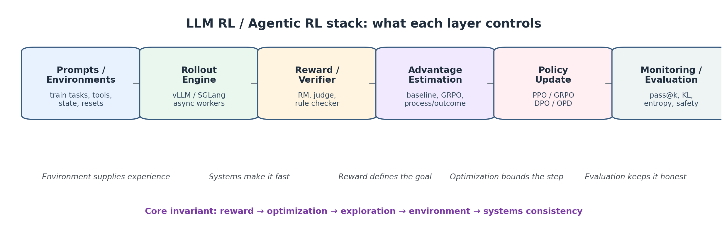 A practical stack view: rewards define the goal, optimization bounds the update, environments supply experience, systems make rollouts fast, and monitoring keeps the whole loop honest.
If you remember only five things:
- RL for LLMs is policy-gradient over generated tokens and trajectories.
- Rewards/verifiers define both the goal and the attack surface.
- GRPO removes the critic by using group-relative baselines.
- RLVR mostly turns latent capability into reliable behavior, unless exploration is preserved long enough.
- Agentic RL is bottlenecked by environments, evaluation, safety, and rollout systems as much as by algorithms.
How to read. Speed-run: read each section’s Key concepts plus the 🎯 one-line answer under every question. Deep: read the full answers and derivations. Math is kept to the few objects you must be able to derive. Every nontrivial claim links to a primary source; see References. A self-test checklist of the original questions is in the Appendix.
Reading paths.
- Interview path: §1–3, §7–9, §12–15, §19, Appendix.
- Reasoning / RLVR path: §1, §5, §8, §10–12, §14.
- Agentic RL path: §13–15, then §16–18 for systems.
- Systems path: §8, §16–18.
Part I — Foundations & Problem Setup
§1 — What post-training is, and the recipe map
Key concepts.
A modern chat/reasoning model is built in two phases. Pre-training learns a base model by next-token prediction on web-scale text — broad knowledge, but no reliable instruction-following or preference for helpful, honest answers. Post-training turns that base model into something usable. It is a recipe of stages, run roughly in this order (Ouyang et al., 2022; Lambert, 2026):
- Instruction tuning / SFT — supervised fine-tuning on (instruction, response) pairs so the model follows instructions and adopts a format/voice (Wei et al., 2021).
- Reward modeling — train a reward model (RM) on human preference pairs to score responses (§4).
- Rejection sampling — sample several responses, keep the best by the RM, fine-tune on them (§6).
- Reinforcement learning — optimize the policy against a reward signal with PPO/GRPO (§7–§8).
- On-policy distillation / direct alignment — cheaper signal sources: distill a teacher on the student’s own rollouts (§6), or skip the RM/RL loop entirely with DPO (§9).
Two reward regimes run through all of this. RLHF (RL from human feedback) uses a learned reward model as a proxy for human preference — flexible, but hackable. RLVR (RL from verifiable rewards) replaces the RM with a programmatic checker — “is the math answer correct?”, “do the unit tests pass?” — which is far harder to game and underpins the reasoning models (DeepSeek-AI, 2025; the term was popularized by Tülu 3, Lambert et al., 2024).
Question: Walk through the standard post-training pipeline — what does each stage actually learn?
🎯 SFT teaches format and instruction-following; the reward model learns human preference; rejection sampling and RL push the policy toward higher-reward behavior; direct-alignment/distillation are cheaper ways to inject the same preference signal.
Each stage fixes a different gap. SFT gets the model to answer in the right shape (follow the instruction, stop at the right place), but it can only imitate demonstrations — it never learns what is better among many valid answers. The reward model captures that relative preference from human comparisons. RL (or rejection sampling) then optimizes the policy to produce responses the reward prefers, exploring beyond the demonstration set. Direct alignment (DPO) and on-policy distillation are alternative ways to deliver preference/teacher signal without standing up the full online RL loop. In practice teams mix these — e.g. SFT → DPO for cheap alignment, then GRPO/RLVR where a verifiable reward exists.
Question: RLHF vs RLVR — when do you not need a reward model?
🎯 When the reward is verifiable. If correctness can be checked programmatically (math, code, format), use that checker directly (RLVR) and skip the learned RM, which removes a whole failure mode (reward-model hacking).
A learned RM is necessary when “good” is subjective — helpfulness, tone, safety — because there is no program that scores it. But for tasks with a ground-truth check (a math answer, passing tests, a regex on format), a verifiable reward is cheaper and often more robust than a learned RM because it removes reward-model overoptimization (DeepSeek-AI, 2025). The verifier is still an attack surface: weak tests, shallow regexes, or leaky environments can still be exploited. The cost is that verifiable rewards are sparse and binary (right/wrong), which is exactly why exploration and difficulty-vs-trainability (§14) become central in RLVR.
Question (added): How much SFT is enough before switching to RL/GRPO?
🎯 Enough SFT means the model can reliably produce valid, scoreable rollouts in the right format, with nontrivial success and failure under the verifier. Once rollouts are mostly parseable and the reward has variance, switch to RL; more SFT is not automatically better because it pulls the model toward a fixed external distribution and can reduce exploration.
The purpose of SFT before RL is bootstrapping, not perfection. It should teach the model the task format, tool/API syntax, stopping behavior, and basic instruction-following so that RL rollouts are not all invalid. A practical readiness checklist:
- Format validity: most outputs are parseable / executable / tool-call-valid.
- Verifier coverage: the reward can score most rollouts without crashing or returning ambiguous results.
- Reward variance: the model has both successes and failures; all-fail means RL has no useful gradient, all-pass means the task is already solved (§14).
- Exploration still exists: samples are not mode-collapsed into a narrow SFT style; response length and solution strategies still vary.
- No broad regression: SFT did not obviously destroy neighboring capabilities you need.
This is the distributional view of the SFT → RL handoff: SFT pulls the policy toward a fixed external target distribution; RL updates on the model’s own rollouts and moves probability mass toward rewarded behavior; OPD sits in between, using on-policy data with a dense teacher signal (wh, 2026). So the handoff point is when the model can generate useful on-policy data. Past that point, additional SFT often buys less than RL because it keeps imitating a dataset rather than optimizing the task objective.
Case study — VibeThinker. The VibeThinker reports make this handoff very concrete. VibeThinker-1.5B frames SFT as a Spectrum Phase: instead of selecting the checkpoint with the best pass@1, it selects and merges specialist checkpoints that maximize pass@K / solution diversity, creating a broad candidate space for RL. RL is then the Signal Phase, using verifiable rewards to amplify the correct paths from that spectrum (Xu et al., 2025). VibeThinker-3B extends the same idea into a fuller pipeline: curriculum SFT, multi-domain RL, Long2Short Math RL, offline self-distillation, and Instruct RL (Xu et al., 2026). The lesson for this FAQ: the best SFT checkpoint for RL is not necessarily the most greedy-accurate one; it is the one that gives RL a valid, diverse, learnable rollout distribution.
Takeaway. Post-training is a recipe — SFT, reward modeling, rejection sampling, RL, and direct-alignment/distillation — and the single most important fork is learned reward (RLHF) vs verifiable reward (RLVR). SFT should get the model to the point where RL can see a real learning signal; then RL/GRPO should take over. The rest of this post is mostly about steps 4–5 and how they change for agents.
§2 — RL background and the math toolkit
Key concepts.
RL frames learning as an agent acting in a Markov Decision Process (MDP): at state \(s_t\) it takes action \(a_t \sim \pi_\theta(\cdot\mid s_t)\), receives reward \(r_t\), and transitions to \(s_{t+1}\) (Sutton & Barto, 2018). For LLMs the mapping is: the state is the prompt plus tokens generated so far, an action is the next token, and the policy is the model. The goal is to maximize expected return \(J(\theta)=\mathbb{E}_{\tau\sim\pi_\theta}[\sum_t \gamma^t r_t]\).
Two value functions summarize the future: \(V^\pi(s)=\mathbb{E}[\,\text{return}\mid s]\) and \(Q^\pi(s,a)=\mathbb{E}[\,\text{return}\mid s,a]\); their difference is the advantage \(A^\pi(s,a)=Q^\pi(s,a)-V^\pi(s)\) — “how much better than average is this action.” The policy-gradient theorem (Sutton et al., 2000) gives the gradient we actually use, \(\nabla_\theta J=\mathbb{E}[\nabla_\theta\log\pi_\theta(a\mid s)\,A]\), and GAE is how we estimate \(A\) (derived in §7).
Three probability tools recur everywhere in RL training:
- Cross-entropy, KL, entropy, MLE — one identity ties them together (Q below).
- Monte-Carlo estimation — approximate an expectation \(\mathbb{E}_{x\sim p}[f(x)]\) by averaging samples; everything in policy-gradient RL is a Monte-Carlo estimate of a gradient.
- Importance sampling and rejection sampling — two ways to handle “I have samples from the wrong distribution” (Q below).
Question (Algo-2): How do cross-entropy, KL divergence, entropy, and MLE relate?
🎯 One identity: \(\mathrm{CE}(p,q)=H(p)+\mathrm{KL}(p\|q)\). Minimizing cross-entropy or KL over \(q\) is the same thing (since \(H(p)\) is constant in \(q\)); and maximum-likelihood training is exactly minimizing \(\mathrm{KL}(p_{\text{data}}\|p_\theta)\).
Write them out for distributions \(p\) (truth) and \(q\) (model): \(H(p)=-\!\sum_x p\log p,\quad \mathrm{KL}(p\|q)=\sum_x p\log\tfrac{p}{q},\quad \mathrm{CE}(p,q)=-\!\sum_x p\log q.\) Adding and subtracting gives \(\mathrm{CE}(p,q)=H(p)+\mathrm{KL}(p\|q)\). Since \(H(p)\) does not depend on the model \(q\), minimizing cross-entropy loss is minimizing KL to the data. And the maximum-likelihood objective \(\max_\theta \mathbb{E}_{x\sim p_{\text{data}}}[\log p_\theta(x)]\) is, term for term, \(\min_\theta \mathrm{KL}(p_{\text{data}}\|p_\theta)\). So next-token pre-training, the SFT loss, and “minimize KL to the data” are the same objective viewed three ways.
Why it matters for RL. KL is asymmetric — \(\mathrm{KL}(p\|q)\neq\mathrm{KL}(q\|p)\) — and which direction you penalize changes behavior (mode-covering vs mode-seeking). The RLHF KL-to-reference term (§7) and its k3 estimator (§8) are direct consequences of this toolkit.
Question (Algo-4): What are importance sampling and rejection sampling, and how are they used in RL?
🎯 Both are Monte-Carlo techniques for “samples from the wrong distribution.” Importance sampling reweights off-policy samples by a probability ratio (used to reuse slightly-stale rollouts); rejection sampling keeps/drops samples to match a target (used for data filtering / best-of-N).
Importance sampling (IS) estimates \(\mathbb{E}_{x\sim p}[f(x)]\) using samples from another distribution \(q\): \(\mathbb{E}_{p}[f]=\mathbb{E}_{q}[\tfrac{p(x)}{q(x)}f(x)]\). The ratio \(w=p/q\) reweights each sample. This is exactly the \(r_t(\theta)=\pi_\theta/\pi_{\theta_{\text{old}}}\) ratio in PPO/GRPO and the staleness correction in async RL (§18) — they let us reuse rollouts from a slightly older policy. The catch: if \(p\) and \(q\) diverge, the ratios explode and the estimator’s variance blows up — which is why we clip (§7) and bound staleness (§18).
Rejection sampling instead generates candidates and accepts a subset to match a target — in post-training, “sample N responses, keep the ones the reward model likes, fine-tune on them” (Touvron et al., 2023). It is the simplest way to turn a reward into training data, and the conceptual seed of §6. Both are Monte-Carlo at heart: estimate/shape a target distribution from samples you can actually draw.
Takeaway. RL is Monte-Carlo estimation of a policy gradient. The advantage (\(Q-V\)) is the object we estimate, importance sampling lets us reuse off-policy samples (at the cost of variance), and the CE/KL/MLE identity is the thread linking pre-training, SFT, and the KL penalties in RL.
§3 — Algorithm families: value-based, policy-gradient, actor-critic
Key concepts.
Classical RL has three families. Value-based methods (Q-learning, DQN) learn \(Q(s,a)\) and act greedily, \(a=\arg\max_a Q(s,a)\); they never represent a policy explicitly. Policy-gradient methods parameterize the policy \(\pi_\theta\) directly and ascend \(\nabla_\theta J\). Actor-critic keeps an explicit policy (the actor) and also learns a value function (the critic) to reduce the variance of the policy gradient — the basis of PPO. LLM RL is almost entirely policy-gradient / actor-critic, for reasons the questions below make concrete.
Question (Algo-1): Why use actor-critic rather than a pure critic (value-based) method?
🎯 Because LLM generation is a huge sequence-level decision problem with sparse terminal rewards. Single-token argmax over the vocabulary is not the core issue — the core issue is that bootstrapped Q-learning over long text trajectories is impractical and unstable. An explicit policy samples trajectories directly; the critic, when used, is only a variance-reduction device.
A value-based method must learn \(Q(s,a)\) and then bootstrap it through Bellman backups. For LLMs, the one-step action is a token, but the meaningful action is often the whole response or tool trajectory: the reward arrives at the sequence/episode level, while the state space is every possible prefix and tool observation. That makes sequence-level maximization, off-policy bootstrapping, and long-horizon credit assignment brittle. A policy sidesteps this: the model already outputs a distribution over the next token, so we can sample complete trajectories and push their log-probabilities up or down by policy gradient. The critic is still useful — it provides the baseline/advantage that cuts gradient variance — but it is an aid to the actor, not the decision maker. That is the actor-critic compromise PPO is built on. (GRPO, §8, goes further and drops the critic, replacing it with a Monte-Carlo group baseline.)
Common pitfall. “Pure critic” is not wrong everywhere — for small discrete action spaces (games, control) value-based methods are excellent. It is specifically stochastic, sequence-level language generation with sparse trajectory rewards that makes a pure value-based approach a poor fit.
Question: Value-based vs policy-gradient vs actor-critic — when does each break down?
🎯 Value-based: breaks in large/continuous action spaces and only yields a deterministic greedy policy. Pure policy-gradient: unbiased but high variance, sample-inefficient. Actor-critic: combines them — explicit (stochastic) policy with a variance-reducing critic — at the cost of a second model and critic bias.
- Value-based (Q-learning/DQN): sample-efficient with replay, but the \(\arg\max\) kills it on large or continuous actions, and a pure greedy policy is deterministic (bad when you need exploration or calibrated sampling).
- Policy-gradient (REINFORCE): handles any action space and gives a stochastic policy, but the raw estimator has high variance and is sample-hungry.
- Actor-critic (PPO): the critic’s value estimate provides a baseline that slashes variance while keeping the explicit policy — the practical default — but you now train and store a critic, and a biased critic biases the advantage.
Takeaway. LLM RL lives in the policy-gradient / actor-critic world because language generation is a stochastic, sequence-level decision problem with sparse trajectory rewards. Keep the explicit policy; treat the critic as a variance-reduction tool — and note that GRPO replaces it with a group baseline (§8).
Part II — Rewards & Preferences
§4 — Preferences and reward modeling
Key concepts.
When “good” is subjective, we cannot write a reward function — we learn one from human comparisons. The standard pipeline collects preference pairs: for a prompt \(x\), a human (or AI) judges response \(y_w\) better than \(y_l\). A reward model (RM) \(r_\phi(x,y)\) — usually the base model with a scalar head — is trained so that preferred responses score higher, via the Bradley–Terry model (Bradley & Terry, 1952), which says the probability that \(y_w\) beats \(y_l\) is
\[P(y_w \succ y_l \mid x) = \sigma\!\big(r_\phi(x,y_w) - r_\phi(x,y_l)\big),\]so the RM is trained by minimizing \(-\log\sigma(r_\phi(x,y_w)-r_\phi(x,y_l))\) (Ouyang et al., 2022). Only differences are learned, so the reward scale is arbitrary (this matters for normalization later).
Beyond a learned scalar RM, two cheaper preference sources are now common:
- LLM-as-judge — prompt a strong model to compare/score responses (Zheng et al., 2023). Cheap and flexible, but biased.
- Rubric / Constitutional feedback — score against an explicit written rubric or constitution (Bai et al., 2022), improving consistency and interpretability.
| Reward source | Cost | Strength | Main weakness |
|---|---|---|---|
| Learned scalar RM | medium (collect prefs + train) | dense, fast at inference | overoptimization, distribution shift |
| LLM-as-judge | low | flexible, no training | position/verbosity/self bias, miscalibration |
| Rubric / constitutional | low–medium | consistent, auditable | rubric design effort |
| Verifiable checker (§5) | low (if checkable) | lower attack surface, exact | only for verifiable tasks; verifier can be exploited |
Table T3. Reward/verifier sources and trade-offs.
Question: How is a reward model trained, and why does only the difference in scores matter?
🎯 Train it on preference pairs with a Bradley–Terry (logistic) loss on the score difference; because the loss only sees \(r(y_w)-r(y_l)\), the absolute scale and offset are unidentifiable — the RM learns relative quality, not an absolute score.
The RM is the base transformer with its LM head replaced by a single scalar output. For each pair we push \(r_\phi(x,y_w)\) above \(r_\phi(x,y_l)\) through the logistic loss above. Two consequences follow directly: (1) adding a constant to all rewards changes nothing, so downstream RL must use a baseline or normalization (this is why GRPO standardizes within a group, §8); (2) the RM is only reliable on the distribution it was trained on — push the policy far from that and the RM’s scores become unreliable, the root of overoptimization (§5).
Question: What goes wrong with LLM-as-judge, and how do you harden it?
🎯 Judges have systematic biases — position, verbosity, self-preference — and are often miscalibrated. Harden with randomized ordering, reference answers/rubrics, pairwise rather than absolute scoring, and calibration checks against human labels.
Zheng et al., 2023 documented that LLM judges prefer the first option (position bias), longer answers (verbosity bias), and outputs from the same model family (self-bias). Practical mitigations: swap order and average, force a rubric or reference answer, prefer pairwise comparison over absolute 1–10 scores (more stable), constrain the output format, and periodically measure judge–human agreement so you know the judge’s calibration. Also: version and freeze the judge prompt during a run. If the judge changes mid-training, the reward target moves and the reward curve becomes uninterpretable. None of this removes bias fully, which is why high-stakes RL leans on verifiable rewards where possible (§5).
Takeaway. Reward modeling converts human preference into a trainable score via Bradley–Terry; its defining limitations — arbitrary scale and reliability only in-distribution — directly motivate normalization (§8) and the verifiable-reward turn (§5).
§5 — Verifiable rewards, regularization, and reward hacking
Key concepts.
A reward is only as good as its resistance to being gamed. Reward hacking (a.k.a. specification gaming) is when the policy maximizes the measured reward without achieving the intended goal — a classic, general RL failure (Amodei et al., 2016; Skalse et al., 2022). With a learned RM this is acute: optimize hard enough and the policy finds the RM’s blind spots, so measured reward rises while true quality falls — reward-model overoptimization, which Gao et al., 2023 showed follows a predictable scaling curve (true reward goes up, peaks, then declines as KL from the reference grows).
Two defenses:
- Verifiable rewards (RLVR). Where correctness is checkable — math answers, unit tests, format regex — score with the checker instead of an RM. This reduces the attack surface, but it moves the attack surface onto the verifier itself (DeepSeek-AI, 2025; Lambert et al., 2024).
- KL regularization. Penalize divergence from a frozen reference policy so the model cannot wander into RM blind spots (§7’s KL-to-reference). This bounds the destination, trading a little reward for staying in-distribution.
The catch: verifiable ≠ unhackable. Test suites can be satisfied by degenerate solutions, format rewards by empty reasoning, and “judge” verifiers by sycophantic phrasing. The reward/verifier is the real attack surface of the whole system.
Question (Algo-3): How should you design rewards for different RL settings?
🎯 Match the reward to what you can actually verify. Prefer a programmatic verifiable reward when the task has ground truth; use a learned RM (or LLM-judge/rubric) only for genuinely subjective qualities; and always design against the cheapest exploit, not just the intended behavior.
A useful checklist when designing a reward:
- Is it verifiable? Math/code/format ⇒ use the checker (cheap, robust). Subjective ⇒ RM or rubric.
- Is it dense or sparse? Verifiable rewards are usually binary/sparse (right/wrong), which makes exploration and curriculum (§14) the bottleneck; RM rewards are dense but hackable.
- What’s the cheapest way to cheat? Long-but-wrong answers (length bias), guessing the format, exploiting judge biases — shape or filter these out (DAPO’s overlong shaping, §8, is exactly this).
- Multi-objective? Combining helpfulness + safety + verifiability invites whack-a-mole; weight explicitly and monitor each term.
For agents specifically, rewards span outcome (did the task succeed?) and process (were the intermediate steps valid?) — outcome rewards are cleaner but sparser; process rewards are denser but re-introduce a learned-verifier attack surface.
Question: How do you detect reward hacking in practice?
🎯 Watch for the tell-tale divergence: measured reward keeps rising while held-out quality stalls or drops. Concrete signals — sudden reward jumps, response-length blow-ups, KL-from-reference spiking, and qualitative inspection of high-reward samples.
Because overoptimization is a gap between proxy and truth (Gao et al., 2023), you detect it by tracking both: proxy reward (RM/verifier score) and an independent signal (held-out verifiable eval, human spot-checks). Operational red flags: reward stepping up discontinuously (found an exploit), mean generation length ballooning (length hacking), KL-to-reference climbing fast (drifting out of distribution), and — the cheapest and most underrated — reading examples. Audit the top-\(k\) highest-reward rollouts (where hacks concentrate) and a random sample (to catch quiet regressions). Mitigations: stronger/ensembled verifiers, KL leash, early stopping on the held-out signal, and removing the exploited shortcut.
Takeaway. The reward/verifier is the system’s attack surface. Verifiable rewards shrink it, KL regularization bounds drift, but nothing is unhackable — monitor the proxy-vs-truth gap continuously.
§6 — Rejection sampling and on-policy distillation
Key concepts.
Not every preference signal needs the full online RL loop. Two lighter-weight techniques sit between SFT and PPO/GRPO.
Rejection sampling (a.k.a. best-of-N fine-tuning). Sample \(N\) responses per prompt from the current model, score them (RM or verifier), keep the best, and fine-tune on those with the ordinary SFT loss (Touvron et al., 2023). It is the simplest way to turn a reward into improvement — no critic, no clipping, no importance sampling — and is a strong, stable baseline. Its limit: it only ever imitates the best of what the current model can already produce, so it cannot explore as far as on-policy RL.
On-policy distillation (OPD). A teacher provides a dense signal on the student’s own rollouts: the student generates a trajectory, and the teacher scores/relabels it token-by-token (e.g. teacher log-probs as the target), which the student distills against (Agarwal et al., 2023, generalized knowledge distillation). The key word is on-policy: unlike vanilla distillation on a fixed corpus, the student learns to fix its own mistakes in the states it actually visits, which closes the train/test distribution gap that plagues off-policy distillation.
Question (Algo-17): How does on-policy distillation improve on plain RL or plain SFT, and where is it used?
🎯 It combines RL’s on-policy exploration with SFT’s dense, low-variance signal: the student samples its own trajectories (like RL) but learns from a teacher’s per-token targets (like SFT) instead of a sparse scalar reward — cheaper and more stable than RL, less distribution-mismatched than off-policy distillation.
Plain SFT (or off-policy distillation) trains on a fixed set of trajectories, so the model never practices recovering from its own errors — at test time it drifts into states the data never covered. Plain RL fixes the distribution problem (it’s on-policy) but its reward is sparse and high-variance, making it expensive and finicky. OPD takes the best of both: on-policy rollouts (correct distribution) + a dense teacher signal (low variance). It is attractive for capability transfer — distilling a large/strong teacher into a smaller student cheaply — and as a warm-start or complement to RLVR. The main requirement is access to a suitable teacher (and, ideally, its token-level distributions; closed APIs that hide logits limit this).
Question (added): What is the difference between rejection-sampling fine-tuning and inference-time best-of-N?
🎯 Same operation, different place. Inference-time best-of-N spends compute at test time and returns the best sample; rejection-sampling fine-tuning uses best-of-N to create new training data, then changes the model weights so future samples improve without paying the test-time cost every time.
Both sample \(N\) candidates and select with a reward/judge/verifier. Best-of-N at inference is a test-time scaling method (§11): no weights change, quality improves only for this request, and latency cost grows with \(N\). Rejection-sampling fine-tuning is a training data generation method: select the good candidates, then run SFT on them. It amortizes the selection cost into the weights, but it is bounded by what the current policy can already sample — if the good behavior never appears in the \(N\) candidates, the model cannot learn it from rejection sampling alone.
Takeaway. Before (or alongside) full RL, rejection sampling and on-policy distillation deliver much of the gain at a fraction of the complexity — rejection sampling by keeping the best of N, OPD by distilling a teacher on the student’s own trajectories.
Part III — Policy Optimization Algorithms
§7 — The PPO family and trust regions
Key concepts.
Reinforcement learning for language models optimizes a policy \(\pi_\theta\) (the model) to maximize expected reward. The workhorse is the policy gradient: instead of differentiating through a reward we cannot differentiate, we push up the log-probability of actions that turned out better than expected. For a trajectory \(\tau\),
\[\nabla_\theta J(\theta) \;=\; \mathbb{E}_{\tau \sim \pi_\theta}\!\left[\sum_t \nabla_\theta \log \pi_\theta(a_t \mid s_t)\, \hat{A}_t \right],\]where \(\hat{A}_t\) is an advantage — how much better action \(a_t\) was than the policy’s average at state \(s_t\). This is the REINFORCE estimator (Williams, 1992) made practical by the policy-gradient theorem (Sutton et al., 2000). Using the advantage instead of the raw return is the single most important variance-reduction trick; estimating it well is the job of GAE (below).
The problem with vanilla policy gradients is step size: one large, badly-scaled update can move the policy into a region where its own samples are no longer informative, and training collapses. Trust-region methods fix this by limiting how far each update may move the policy. TRPO (Schulman et al., 2015a) makes this explicit — maximize the reward subject to a hard KL constraint:
\[\max_\theta\; \mathbb{E}_t\!\left[ r_t(\theta)\, \hat{A}_t \right] \quad \text{s.t.} \quad \mathbb{E}_t\!\left[ \mathrm{KL}\big(\pi_{\theta_{\text{old}}}(\cdot\mid s_t)\,\|\,\pi_\theta(\cdot\mid s_t)\big) \right] \le \delta,\]where \(r_t(\theta) = \dfrac{\pi_\theta(a_t \mid s_t)}{\pi_{\theta_{\text{old}}}(a_t \mid s_t)}\) is the importance-sampling ratio that lets us reuse samples from the slightly-older policy \(\pi_{\theta_{\text{old}}}\).
PPO (Schulman et al., 2017) replaces the hard constraint with a cheap clipped surrogate objective that approximates the trust region with first-order methods:
\[L^{\text{CLIP}}(\theta) \;=\; \mathbb{E}_t\!\left[ \min\!\Big( r_t(\theta)\,\hat{A}_t,\;\; \mathrm{clip}\big(r_t(\theta),\, 1-\epsilon,\, 1+\epsilon\big)\,\hat{A}_t \Big) \right].\]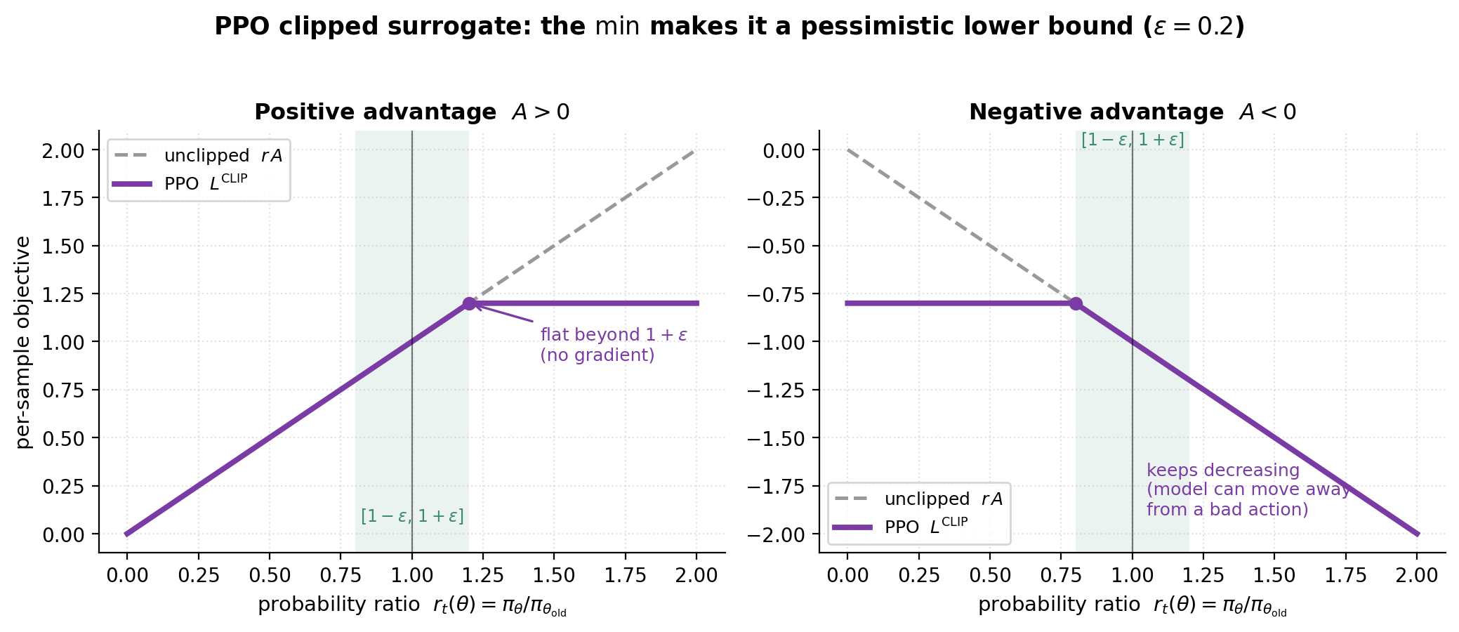 The clipped surrogate for \(A>0\) (left) and \(A<0\) (right). Inside \([1-\epsilon,1+\epsilon]\) it follows the unclipped \(rA\); outside, the outer \(\min\) flattens the upside (left) while still letting the policy move away from bad actions (right). This asymmetry is exactly what makes \(L^{\text{CLIP}}\) a pessimistic lower bound.
The advantage is typically estimated with Generalized Advantage Estimation (Schulman et al., 2015b):
\[\hat{A}_t^{\mathrm{GAE}(\gamma,\lambda)} = \sum_{l=0}^{\infty} (\gamma\lambda)^l\, \delta_{t+l}, \qquad \delta_t = r_t + \gamma V(s_{t+1}) - V(s_t),\]which interpolates between low-variance/high-bias (\(\lambda\to 0\)) and high-variance/low-bias (\(\lambda\to 1\)) advantage estimates.
In RLHF, PPO does not optimize the raw reward model score. It optimizes the reward model minus a KL penalty to a frozen reference policy, which keeps the model from drifting into degenerate, reward-hacking text (Stiennon et al., 2020; Ouyang et al., 2022):
\[R(x,y) \;=\; r_\phi(x,y) \;-\; \beta\, \mathrm{KL}\big(\pi_\theta(\cdot\mid x)\,\|\,\pi_{\text{ref}}(\cdot\mid x)\big).\]This PPO recipe — actor + critic + reward model + reference model — is the canonical RLHF setup (Lambert, 2026, Policy Gradient chapter). It is powerful but memory-heavy (four models in play); the next section (§8, GRPO) is largely a reaction to that cost.
Question: What is PPO’s clipping actually defending against, and where does the min come from?
🎯 Clipping caps how much one update can change the policy per token; the outer min makes the objective a pessimistic lower bound so the update only “trusts” changes inside the clip range.
Vanilla policy gradients can take a destructively large step when the importance ratio \(r_t(\theta)\) drifts far from 1 — exactly the failure TRPO’s KL constraint was designed to prevent (Schulman et al., 2015a). PPO approximates that trust region without the expensive constrained optimization. Two pieces do the work:
-
clip(r, 1-ε, 1+ε)removes the incentive to push the ratio beyond \([1-\epsilon, 1+\epsilon]\) (typically \(\epsilon\approx 0.2\)): once you are outside the band, the clipped term is flat, so its gradient is zero and the update stops pushing. - The outer
minbetween the unclipped and clipped terms makes the surrogate a lower bound on the true objective. This matters for the sign of the advantage: when \(\hat{A}_t > 0\) it caps the upside of increasing the probability; when \(\hat{A}_t < 0\) it still lets the model move away from a bad action. Without themin, clipping alone would let the policy over-correct on negative-advantage samples (Schulman et al., 2017).
What if you don’t clip? A single token whose ratio drifts far from 1 produces an unbounded \(r_t\hat{A}_t\) term, so one minibatch can take a huge, badly-scaled step; the policy moves into a region where its old samples are off-distribution, the importance weights become unreliable, and training destabilizes or collapses. Clipping is the cheap guard against that.
Common pitfall. Clipping bounds the per-update step, not cumulative drift. Over many epochs the policy can still wander far from \(\pi_{\text{ref}}\), which is why RLHF keeps a separate KL-to-reference penalty in the reward (above). Clip and KL-to-ref solve different problems — one bounds the step, the other bounds the destination.
Question: What does CISPO change about PPO/GRPO clipping, and why?
🎯 PPO/GRPO clipping makes the objective flat in the reward-improving direction once the ratio crosses the clipped side; CISPO instead clips the importance-sampling weight while keeping the log-prob gradient flowing through every token, preserving rare-but-pivotal updates.
The subtle cost of PPO-style clipping is which tokens get clipped. In long chain-of-thought, the tokens with large ratios are often the rare, high-information ones — reflective/branching tokens like “wait”, “but”, “alternatively” — and zeroing their gradient throws away exactly the updates that teach reasoning. CISPO (Clipped IS-weight Policy Optimization), introduced in MiniMax-M1 (2025), keeps the REINFORCE-style term \(\texttt{sg}(w_t)\,\hat{A}_t\,\nabla_\theta \log \pi_\theta(a_t\mid s_t)\) but clips the importance-sampling weight \(w_t\) (a stop-gradient multiplier) instead of clipping the objective. Because the clip lands on the weight, not on the log-prob gradient, all tokens keep contributing gradient — the trust-region bound is preserved (via the weight) without silencing high-ratio tokens. MiniMax-M1 reports this is both more stable and more sample-efficient for long-reasoning RL.
If asked in an interview: “PPO-style clipping can stop reward-improving updates once a token’s ratio crosses the clipped side; CISPO clips the IS weight instead, so the log-prob gradient still flows, with bounded weight.”
| Method | What it bounds | How it’s enforced | Effect once outside the clipped side |
|---|---|---|---|
| TRPO (2015a) | KL\((\pi_{\text{old}}|\pi_\theta)\le\delta\) | hard constraint (CG + line search) | n/a (constrained step) |
| PPO (2017) | per-token ratio \(\in[1-\epsilon,1+\epsilon]\) | clip the objective, take min | may become flat in the reward-improving direction |
| CISPO (2025) | the IS weight \(w_t\) | clip the weight, keep log-prob gradient | gradient still flows, with bounded weight |
Question: TRPO vs PPO vs the “staleness bound” in async RL — how are they the same idea?
🎯 All three bound how far the behavior (sampling) policy may diverge from the policy being updated; they differ only in how the bound is enforced.
- TRPO: a hard KL constraint solved with constrained optimization (conjugate gradient + line search) (Schulman et al., 2015a). Most faithful, most expensive.
- PPO: an approximate trust region via clipping the ratio — first-order, cheap, the practical default (Schulman et al., 2017).
- Async RL staleness bounds: in asynchronous setups the rollouts are generated by a policy that is already a few steps behind the trainer, so the data is off-policy. Frameworks bound this gap (e.g. a max number of off-policy steps) and correct the residual with importance sampling — conceptually the same “don’t stray too far” budget, but enforced over wall-clock staleness rather than per-update (Fu et al., 2025, AReaL). We return to staleness in §18.
If asked in an interview: “They are all trust regions. TRPO enforces it exactly, PPO approximately via clipping, async RL enforces a staleness budget plus importance-sampling correction.”
Question (added — not in the source set, but worth knowing): Why optimize the advantage instead of the raw reward/return, and what do γ and λ trade off in GAE?
🎯 Subtracting a baseline to form the advantage cancels the high-variance part of the gradient that does not depend on the action; γ and λ then trade bias against variance in estimating it.
The policy-gradient estimator is unbiased with any state-dependent baseline \(b(s)\): \(\mathbb{E}[\nabla\log\pi_\theta(a|s)\,b(s)] = 0\). Choosing \(b(s)=V(s)\) gives the advantage \(A = Q - V\), which has much lower variance than the raw return because it measures relative quality of an action, not the absolute (and noisy) return (Sutton et al., 2000). GAE (Schulman et al., 2015b) then estimates \(A\) as an exponentially-weighted sum of TD residuals: \(\gamma\) discounts future reward (problem definition), while \(\lambda\) controls the bias–variance trade-off of the estimator — small \(\lambda\) trusts the learned value function \(V\) (low variance, biased if \(V\) is wrong), large \(\lambda\) trusts the empirical returns (high variance, low bias).
Insight box — “Clip and KL solve different problems.” The PPO clip bounds one step; the KL-to-reference term bounds the final destination relative to the base model. Reasoning-focused RLVR runs often drop the KL-to-reference (to let the policy move far enough to learn new behavior) while keeping the clip for stability — see §5 and §8.
Takeaway. PPO is an approximate trust region: the clip bounds each update, GAE supplies a low-variance advantage, and (in RLHF) a separate KL-to-reference term anchors the policy to the base model. Almost every later LLM-RL algorithm is a modification of this template.
§8 — GRPO and the variant zoo
Key concepts.
PPO’s biggest practical cost is the critic: a second network, about the size of the policy, that must be trained alongside it to estimate \(V(s)\) for the advantage. GRPO (Group Relative Policy Optimization), introduced in DeepSeekMath (Shao et al., 2024) and made famous by DeepSeek-R1 (DeepSeek-AI, 2025), removes the critic entirely. The idea: for each prompt, sample a group of \(G\) responses, score them, and use the group as its own baseline. The advantage of response \(i\) is just its reward standardized within the group:
\[\hat{A}_{i} \;=\; \frac{r_i - \mathrm{mean}(r_1,\dots,r_G)}{\mathrm{std}(r_1,\dots,r_G)}.\]Everything else looks like PPO — the same clipped ratio — but with this group-relative advantage and (in the original formulation) a KL-to-reference penalty added directly to the loss rather than folded into the reward:
\[\mathcal{J}_{\text{GRPO}}(\theta) = \mathbb{E}\!\left[ \frac{1}{G}\sum_{i=1}^{G} \frac{1}{|o_i|}\sum_{t} \min\!\big(r_{i,t}\hat{A}_i,\ \mathrm{clip}(r_{i,t}, 1\pm\epsilon)\hat{A}_i\big) \;-\; \beta\,\mathbb{D}_{\text{KL}}\!\big[\pi_\theta \,\|\, \pi_{\text{ref}}\big] \right].\]The KL term uses the low-variance, always-positive k3 estimator (Schulman, 2020): \(\mathbb{D}_{\text{KL}} \approx \tfrac{\pi_{\text{ref}}}{\pi_\theta} - \log\tfrac{\pi_{\text{ref}}}{\pi_\theta} - 1\).
This trade — a learned critic for a Monte-Carlo group baseline — is why GRPO became the default for RLVR/reasoning: it is cheaper, simpler, and works well when you can afford several rollouts per prompt. The “variant zoo” (Table T1) is then a sequence of small fixes to GRPO’s known biases.
Insight box — “Drop the critic, keep the baseline.” GRPO’s advantage is a baseline-subtracted reward; the group mean replaces the value network. The cost moves from a second model to extra rollouts.
| Method | Year | Key change vs GRPO | Known weakness |
|---|---|---|---|
| GRPO (Shao 2024) | 2024 | group-mean baseline, no critic; KL in loss | std/length biases (below) |
| Dr. GRPO (Liu 2025) | 2025 | removes std- and length-normalization | needs careful reward scaling |
| DAPO (Yu 2025) | 2025 | clip-higher, dynamic sampling, token-level loss, overlong shaping; drops KL | more hyperparameters |
| GSPO (Qwen 2025) | 2025 | sequence-level importance ratio, clipping, and optimization | coarser credit per token |
| CISPO (MiniMax 2025) | 2025 | clip the IS weight, keep all-token gradient (see §7) | weight clipping tuning |
Table T1. The main GRPO variants. Each is a targeted fix to a specific GRPO bias; many more exist, but these four cover the ideas that recur in practice.
Question (Algo-5): How is the GRPO/PPO advantage computed, why subtract a baseline, and must you divide by std?
🎯 Advantage = reward minus a baseline (the group mean in GRPO); subtracting the baseline cancels the high-variance, action-independent part of the gradient. Dividing by std is optional — it stabilizes scale across prompts but introduces a difficulty bias that Dr. GRPO removes.
The baseline question is the same one from §7: for any state-dependent \(b(s)\), \(\mathbb{E}[\nabla\log\pi\,b(s)]=0\), so subtracting it leaves the gradient unbiased but lower-variance. GRPO’s twist is that the baseline is Monte-Carlo: the mean reward of the \(G\) sampled responses, which is why it needs no critic.
The ÷std is not required. It rescales every prompt’s advantages to unit variance, which helps when prompts have very different reward scales. But Liu et al., 2025 (Dr. GRPO) show it introduces a difficulty bias: easy prompts (low reward std) get their advantages blown up, hard prompts shrunk — plus the per-response length normalization \(1/|o_i|\) creates a length bias that rewards longer wrong answers. Dr. GRPO drops both normalizations and reports cleaner optimization.
Common pitfall. When all \(G\) responses get the same reward, \(\mathrm{std}=0\) → division blows up (implementations add ε or skip the group). Worse, that prompt carries zero learning signal (all-same reward ⇒ zero advantage) — the seed of DAPO’s “dynamic sampling” and of the difficulty-vs-trainability point in §14.
Question (Algo-8): Why does GRPO add a KL term, how is it computed, and why do DAPO/GSPO drop it?
🎯 The KL-to-reference anchors the policy to the base model so RL doesn’t degrade general ability; it’s computed with the k3 estimator. RLVR-scale runs (DAPO/GSPO) drop it because, with a verifiable reward, the leash mostly prevents the model from moving far enough to learn.
In RLHF the KL guards against drifting into reward-model blind spots (reward hacking). But in RLVR the reward is a verifiable checker (math/code correctness), which is much harder to hack, so the main effect of the KL leash is to slow down learning of genuinely new reasoning behavior. Empirically, DAPO removes the KL term and trains more aggressively; this is now common for reasoning RL. Computation: the k3 estimator above is preferred over the naive \(\log(\pi_\theta/\pi_{\text{ref}})\) because it is unbiased, always positive, and lower-variance (Schulman, 2020).
If asked in an interview: “KL keeps you near the base model — essential when the reward is a hackable RM, expendable when the reward is verifiable. RLVR runs drop it to learn faster.”
Question (Algo-13): What do the GRPO variants (Dr. GRPO, DAPO, GSPO, CISPO, …) each fix?
🎯 Each patches a specific GRPO bias: Dr. GRPO removes std/length normalization bias; DAPO adds clip-higher + dynamic sampling + token-level loss + overlong handling and drops KL; GSPO moves the importance ratio to sequence level for MoE stability; CISPO clips the IS weight to keep all-token gradients.
- Dr. GRPO — removes the std and length normalizations that bias optimization toward easy/long answers (Liu et al., 2025).
- DAPO — four tricks (Yu et al., 2025): clip-higher (decouple the upper/lower clip \(\epsilon\) to preserve exploration), dynamic sampling (drop prompts where all responses are right or all wrong — no gradient), token-level policy loss, and overlong reward shaping; also drops KL.
- GSPO — Qwen/Alibaba’s Group Sequence Policy Optimization (Qwen Team, 2025) moves GRPO/PPO-style token-level clipping to sequence-level clipping: it defines the importance ratio with sequence likelihood, aligns the optimization granularity with sequence-level rewards, and reports better stability/efficiency for large-scale MoE RL post-training (including Qwen3 improvements).
- CISPO — clips the importance-sampling weight instead of the objective, keeping gradient on every token (see §7; MiniMax, 2025).
Caveat (for the reader). This space moves fast and new variants appear monthly; treat each entry as “the problem it claims to fix” and check the primary source before relying on the exact deltas.
Question (Algo-12): How do you set group size, learning rate, PPO epochs, and generation length?
🎯 Group size 8–16 (bigger = better baseline, more compute); lr ~1e-6 (RL is touchy); PPO epochs ≈ 1 (more reuse = more off-policy = unstable); generation length set to fit the task’s reasoning budget.
| Hyperparameter | Typical | Why |
|---|---|---|
| group size \(G\) | 8–16 | larger ⇒ lower-variance group baseline, but linearly more rollout cost |
| learning rate | ~1e-6 (policy) | RL is far more sensitive than SFT; too high ⇒ collapse |
| PPO epochs | 1 (sometimes 2–4) | reusing the same rollouts more makes the data increasingly off-policy → instability |
| generation length | task-dependent | too short truncates reasoning; too long wastes rollout compute and invites length hacking |
Table T2. Sensible GRPO defaults. These are starting points, not laws — verify per task.
Takeaway. GRPO swaps PPO’s critic for a group-mean baseline; the variant zoo (Dr. GRPO, DAPO, GSPO, CISPO, …) is a catalog of patches for its std/length/KL/credit biases. Know the bias each one targets, not just its name.
Minimal GRPO runbook.
for prompts in batches:
    # 1. Roll out from the behavior policy and SAVE old logprobs.
    responses, old_logprobs, policy_mask = rollout(
        policy_behavior, prompts, group_size=G
    )

    # 2. Score each response/trajectory with a verifier or reward model.
    rewards = verifier(prompts, responses)

    # 3. Compute group-relative advantages per prompt.
    adv = rewards - rewards.mean(group="prompt")  # std normalization optional

    # 4. Recompute logprobs under the train policy.
    new_logprobs = policy_train.logprob(prompts, responses)
    ratio = exp(new_logprobs - old_logprobs)

    # 5. Apply clipped policy-gradient loss only on policy-generated tokens.
    loss = -masked_mean(
        min(ratio * adv, clip(ratio, 1-eps, 1+eps) * adv),
        mask=policy_mask,  # mask prompts, tool outputs, and observations
    )

    # 6. Log what can go wrong.
    log(reward=mean(rewards), group_std=std(rewards),
        entropy=policy_entropy, clip_fraction=frac_clipped,
        length=mean_len, all_pass=all(r == 1 for r in rewards),
        all_fail=all(r == 0 for r in rewards))
§9 — Direct alignment (DPO and friends)
Key concepts.
PPO/GRPO are online: you sample from the current policy, score, and update. Direct alignment asks whether we can skip the reward model and the sampling loop entirely and just optimize on a fixed set of preference pairs. DPO (Direct Preference Optimization, Rafailov et al., 2023) shows you can. The trick is algebraic: the KL-regularized RLHF objective has a known closed-form optimum,
\[\pi^*(y\mid x) \;\propto\; \pi_{\text{ref}}(y\mid x)\,\exp\!\Big(\tfrac{1}{\beta} r(x,y)\Big),\]which you can invert to write the reward in terms of the policy: \(r(x,y) = \beta \log \tfrac{\pi_\theta(y\mid x)}{\pi_{\text{ref}}(y\mid x)} + \beta\log Z(x)\). Substituting this into the Bradley–Terry preference likelihood makes the partition function \(Z(x)\) cancel, leaving a simple supervised loss on preference pairs \((y_w \succ y_l)\):
\[\mathcal{L}_{\text{DPO}} = -\,\mathbb{E}_{(x,y_w,y_l)}\!\left[ \log \sigma\!\Big( \beta \log \tfrac{\pi_\theta(y_w\mid x)}{\pi_{\text{ref}}(y_w\mid x)} - \beta \log \tfrac{\pi_\theta(y_l\mid x)}{\pi_{\text{ref}}(y_l\mid x)} \Big) \right].\]So DPO’s “reward” is implicit: the quantity \(\beta\log(\pi_\theta/\pi_{\text{ref}})\) is the reward the policy is implicitly being trained against — “your language model is secretly a reward model.” No RM, no rollouts, no online loop; just a contrastive log-likelihood. That simplicity is why DPO is the default for cheap, stable preference tuning.
Question (Algo-10): What is DPO’s reward, can DPO be over-optimized, and how do you fix it?
🎯 DPO’s implicit reward is \(\beta\log(\pi_\theta/\pi_{\text{ref}})\). It has no explicit RM to hack, but the fixed preference objective can still be over-optimized or exploited: likelihood displacement, length exploitation, and off-distribution drift. Fixes: keep an SFT/NLL anchor, length-normalize, use on-policy or iterative preference data, or conservative variants.
DPO has no learned RM to game, so “reward hacking” is not quite the right term. The more precise failure is objective over-optimization: it only sees a fixed, off-policy preference dataset. Three things go wrong in practice:
- Likelihood displacement — the loss only cares about the gap \(\log\pi(y_w)-\log\pi(y_l)\); it can push that gap up while decreasing \(\pi(y_w)\) too, as long as \(\pi(y_l)\) drops faster. The model can become less likely to produce the preferred answer.
- Length / style exploitation — if preferred answers are systematically longer, DPO learns “longer = better” rather than the intended quality signal.
- Distribution shift — because the data is off-policy, DPO can drift to regions the preference set never covers and degrade there.
Mitigations seen in practice: add an SFT (NLL) regularizer on the chosen responses to anchor \(\pi(y_w)\); length-normalize (as in SimPO); move to on-policy / iterative DPO (regenerate preferences from the current policy); or use reformulated objectives — IPO (Azar et al., 2023) to curb over-optimization, KTO (Ethayarajh et al., 2024) to learn from unpaired good/bad labels, SimPO (Meng et al., 2024) to drop the reference model and length-normalize.
Question: DPO vs PPO/GRPO — when do you reach for which?
🎯 DPO when you have a fixed preference set and want cheap, stable tuning with no RM or rollouts; online RL (PPO/GRPO) when you have a reward signal you can query during training — especially a verifiable one — and need exploration beyond the preference data.
DPO trades away the online loop: no reward model to train/serve, no sampling during training, far fewer moving parts — at the cost of being stuck with the preference distribution you started with. PPO/GRPO keep the online loop, so they can explore, use a verifiable reward (RLVR), and improve on prompts no human labeled — at the cost of infrastructure (rollout engine, more models in memory, §16). A common modern recipe: SFT → DPO for cheap alignment, then GRPO/RLVR for reasoning where a verifiable reward exists.
If asked in an interview: “DPO is offline preference optimization with an implicit reward — cheap and stable but bounded by the data; GRPO is online with an explicit (often verifiable) reward — more powerful but more infrastructure. Use DPO for preferences, RLVR for verifiable reasoning.”
Takeaway. DPO collapses RM-training + RL into one contrastive loss via the closed-form RLHF optimum; its implicit reward can still be over-optimized, which the SFT-anchor / length-norm / on-policy / IPO-KTO-SimPO family addresses. Direct alignment and online RL are complementary, not competitors.
Part IV — Reasoning, Test-Time Scaling & Evaluation
§10 — RLVR and reasoning
Key concepts.
The reasoning models (OpenAI o1, DeepSeek-R1) are the headline result of RLVR: take a base model, give it a verifiable reward (math answer correct? tests pass?), and run large-scale RL — and long chain-of-thought, self-correction, and “thinking” emerge (DeepSeek-AI, 2025). The mechanism is simple to state: the policy is rewarded only for correct final answers, and the only way to raise its success rate on hard problems is to generate longer, more careful reasoning — so RL selects for it. Chain-of-thought itself (Wei et al., 2022) is the substrate; RLVR amplifies it.
A central, hotly-debated question is whether RL adds new capability or only sharpens what the base model already has. The evidence leans toward sharpening: Yue et al., 2025 find that RLVR improves pass@1 but often does not expand pass@k at large \(k\) — i.e. RL concentrates probability on solutions the base model could already occasionally sample, rather than discovering genuinely new ones. This connects to two related entropy stories. Entropy collapse studies how reasoning RL can rapidly reduce policy entropy and plateau; The Entropy Mechanism of RL for Reasoning LMs proposes Clip-Cov / KL-Cov to control high-covariance tokens and preserve exploration (Entropy Mechanism, 2025). A complementary line treats entropy as an exploration signal: Reasoning with Exploration finds that high-entropy regions often coincide with turning points, self-verification/correction, and rare reasoning behaviors, and adds a clipped, gradient-detached entropy term to the advantage to encourage exploratory reasoning rather than blindly maximizing policy entropy (Reasoning with Exploration, 2025).
Question (Algo-18): At which training stage does reasoning ability appear?
🎯 The latent ability is laid down in pre-training; RL post-training (RLVR) elicits and amplifies it. RL does not teach math from scratch — it reshapes the base model’s distribution toward reliably using the reasoning it already partially has.
Pre-training on web-scale text (including math, code, and worked solutions) gives the base model the raw ingredients — it can already produce correct chains-of-thought sometimes. SFT teaches the format; RLVR then optimizes for correctness, which pushes the model to deploy reasoning reliably and at length. The strongest evidence that the substrate is pre-existing is the pass@k finding above (Yue et al., 2025): if RL were creating new capability, pass@k would rise at large \(k\); mostly it does not. So: pre-training creates the capability, RL makes it reliable.
Question (Algo-15): Can RL expand an LLM’s capability boundary, or only sharpen it?
🎯 Mostly sharpen, within current methods — RL raises the probability of already-reachable solutions more than it discovers new ones. Whether prolonged/curriculum RL can genuinely expand the boundary is an open research question with early positive signs.
The default finding is “sharpen, not expand” (Yue et al., 2025). But this is method-dependent, not a law: if exploration is kept alive (entropy regularization, diverse data, curriculum) and training is run long enough, there are reports of genuine boundary expansion — see §11’s ProRL discussion. The honest answer for an interview: with standard short GRPO runs, RL sharpens; whether scaled-up, exploration-preserving RL expands the frontier is unsettled and an active area.
Insight box — “pass@1 up, pass@k flat.” The cleanest test of “new ability vs sharpening”: if RL only moves pass@1 but not pass@k, it concentrated existing mass rather than finding new solutions.
Takeaway. RLVR turns verifiable correctness into emergent long-form reasoning, but — within today’s recipes — mostly by sharpening the base model’s existing distribution (pass@1 ↑, pass@k ≈), with entropy collapse as the limiting factor.
§11 — RL vs test-time scaling
Key concepts.
There are two distinct ways to spend compute to get better answers. RL (train-time) reshapes the weights so the model is better on average. Test-time scaling (TTS) spends more inference compute on a fixed model — longer chains-of-thought, sampling many solutions and selecting (best-of-N, majority vote), or search — to get a better answer on this particular query (Muennighoff et al., 2025; OpenAI o1, 2024). They are complementary: RL raises the curve, TTS moves along it at inference.
Their exploration differs too (Algo-6). RL explores in weight space over training — it samples trajectories, and the reward gradient slowly moves the policy toward regions of higher expected reward; exploration is governed by policy entropy and is consumed as entropy collapses (§10). TTS explores in output space at inference — for one prompt it samples diverse candidates (high temperature, many rollouts) and selects, with no weight change; its “exploration” is bounded by the model’s current distribution and the inference budget.
Question (Algo-6): How do RL training and test-time scaling each explore?
🎯 RL explores across training by sampling trajectories and shifting the policy toward high-reward regions (exploration limited by policy entropy, spent over many steps). TTS explores at inference by drawing many diverse samples for a single query and selecting among them (no weight update, limited by the inference budget and the current model’s diversity).
Put concretely: in RL, exploration is “try many trajectories over thousands of updates, keep what the reward likes” — its currency is entropy over training, and when entropy collapses the model stops finding new behavior. In TTS, exploration is “for this one question, think longer or sample 64 answers and take the majority/best” — its currency is inference compute now, and it cannot exceed what the fixed model can already express. This is why the two compose well: use RL to make the per-sample distribution good, then use TTS to cash in extra inference compute on hard queries.
Question (Algo-16): How do you scale the RL training frontier (cf. ProRL)?
🎯 Keep exploration alive and train much longer. ProRL-style results suggest that with entropy control, KL resets, diverse/curriculum data, and prolonged training, RL can reach reasoning the base model does not show even at high pass@k — pushing beyond the “sharpening only” regime.
ProRL (Liu et al., 2025) argues the “RL only sharpens” finding is partly an artifact of short training. Its recipe for scaling the frontier is long, stable RL: KL-divergence control, periodic reference-policy / optimizer reset, diverse verifiable tasks, dynamic sampling, higher rollout temperature, and a multi-task verifiable corpus (math, code, STEM, logic puzzles, instruction following). The key claim is not merely pass@1 improvement: prolonged RL can, on some tasks, discover reasoning strategies that the base model fails to reach even with large sampling. The paper also makes the caveat we should keep in mind: the effect is task-dependent, and gains on a math benchmark’s pass@1 do not automatically imply pass@128 or frontier expansion everywhere. The general lesson for scaling RL is still clear: the binding constraint is usually exploration/diversity, not raw compute — protect entropy, reset the reference when needed, and feed a curriculum (ties directly to §14).
Question (Algo-19): From DeepSeek-R1 to V3/V3.2/V4 — what changed in the RL, and what’s different about MoE RL?
🎯 DeepSeek-R1 made large-scale RLVR on an MoE base visible; V3.2 moved toward specialist distillation plus mixed RL with GRPO and MoE-specific stabilizers; V4 publicly appears to separate domain-expert cultivation (SFT+GRPO) from unified model consolidation via OPD. MoE RL is harder because expert routing makes training–inference consistency and per-token ratios fragile.
At a high level, R1 demonstrated large-scale RLVR for reasoning on top of a V3 MoE base (DeepSeek-AI, 2025). V3.2 reports a post-training recipe built from specialist distillation + mixed RL training: train specialists, then mix reasoning / agent / human-alignment data into a final RL stage, still using GRPO, to avoid catastrophic forgetting from many isolated stages. For reasoning and agent tasks, the reward is mostly rule-based outcome reward plus shaping such as length penalty and language-consistency reward; general tasks use a generative RM with per-prompt rubrics. The reported scaling stabilizers include unbiased KL estimates, off-policy sequence masking, Keep Routing, and Keep Sampling Mask. Keep Routing is especially relevant for MoE RL: it saves the expert routing used during rollout and reuses it during training to reduce router mismatch (DeepSeek-V3.2, 2025).
V4 should be described more carefully. Public materials characterize its post-training as a two-stage pipeline: first cultivate domain experts (e.g. math, coding, agent, instruction following) with SFT + GRPO, then consolidate those capabilities into a unified student via on-policy distillation (OPD) using the student’s own trajectories and teacher signals (DeepSeek, 2026; DeepSeek-V4, 2026; NVIDIA model card, 2026). The safe claim is not that V4 replaces GRPO with a wholly new RL algorithm; rather, expert-stage RL still uses GRPO, while the final unification relies heavily on OPD. Reward formulas, KL/clip hyperparameters, rollout batch settings, the full teacher list, and many OPD engineering details are not fully public.
What is robustly true is why MoE makes RL harder:
- Routing nondeterminism — which experts fire can differ between the rollout (inference) engine and the trainer, so the same tokens get different probabilities → broken importance ratios (this is the MoE training–inference mismatch of §18, Algo-11).
- Token-level ratio noise — per-token IS ratios are noisier under routing, which motivates sequence-level importance sampling (GSPO, §8).
- Expert parallelism — sharding experts adds all-to-all communication and load-balance concerns to the training system (§16).
Takeaway. RL (weights) and test-time scaling (inference) are complementary compute levers; scaling the RL frontier is mostly an exploration problem (ProRL); and MoE models make RL a systems problem, chiefly via routing-induced training–inference mismatch.
§12 — Evaluation: how do you know RL actually helped?
Key concepts.
RL is easy to fool yourself with. A training reward curve going up is not enough: maybe the model found a verifier exploit, got longer, overfit the public tests, or improved only under a larger test-time budget. Evaluation has to separate training signal, held-out capability, exploration, and systems health. The cleanest question is: under a fixed inference budget and a held-out verifier, does the trained policy solve more tasks without regressions elsewhere?
All model comparisons should be budget-controlled: same prompts, same decoding settings, same sampling count, same tool limits, and the same inference budget. Otherwise you may be measuring “spent more test-time compute” rather than “the model got better.”
For reasoning, always separate pass@1 from pass@k / best-of-N / majority vote. Pass@1 measures how much probability mass the policy puts on a correct solution; pass@k measures whether a correct solution exists somewhere in the model’s distribution. This distinction is exactly what lets you test “sharpening vs frontier expansion” (§10). For agents, also measure trajectory properties: success rate, turn count, tool errors, side effects, cost per success, and environment reset failures.
Question (added): How do you evaluate whether an RL run improved the model rather than overfit the verifier?
🎯 Use a held-out, contamination-controlled eval under a fixed inference budget; track pass@1/pass@k, reward, KL/entropy/length, and manually audit top-reward and random samples. If reward rises but held-out quality stalls or drops, you optimized the proxy, not the task.
A minimal evaluation protocol:
- Capability: held-out pass@1, pass@k, best-of-N / majority-vote with a fixed sampling budget.
- Training health: reward curve, held-out verifier score, KL-to-ref, entropy, clip fraction, ratio distribution, response length, advantage distribution.
- Data split: no train/test environment leakage; hidden tests where possible; verifier unavailable to the generator when creating training data.
- Agent metrics: task success, average turns, tool-call count, tool error/timeout rate, side-effect rate, cost per success.
- Judge reliability: if using LLM-as-judge, freeze the judge prompt, randomize order, and track human agreement (§4).
The key is triangulation. A single metric is easy to hack; a run is convincing when reward, held-out success, entropy/KL, length, and qualitative audits all tell the same story.
Question (added): What should you log during a real GRPO/RLVR run?
🎯 Log enough to diagnose reward hacking, entropy collapse, off-policyness, and systems starvation: reward, KL, entropy, clip fraction, ratio distribution, length, group reward std, all-pass/all-fail rate, rollout throughput, trainer idle time, queue size, staleness, and held-out quality.
| Layer | Metrics to log | What they catch |
|---|---|---|
| Policy | reward, KL, entropy, clip fraction, ratio distribution, grad norm | collapse, too-large updates, loss of exploration |
| Generation | length, truncation rate, tool-call count, timeout rate | overlong hacking, bad caps, tool instability |
| Data | all-pass/all-fail fraction, group reward std, prompt repeat rate | no learning signal, duplicate tasks |
| Systems | rollout tokens/s, trainer idle time, queue size, staleness distribution, KV-cache utilization | rollout bottlenecks, async instability |
| Quality | held-out pass@1/pass@k, human spot checks, top-reward audit | proxy overfit, reward hacking |
Takeaway. Evaluation is not a leaderboard number. It is a dashboard that separates proxy reward from true capability, train from test, pass@1 from pass@k, and model quality from systems bottlenecks.
Part V — Agentic RL
§13 — From single-turn RLHF to multi-turn agentic RL
Key concepts.
Everything so far assumed a single turn: prompt in, one response out, one reward. An agent is different — it acts over many steps in an environment: call a tool, read the result, decide the next action, repeat, until a task is done. RL for agents keeps the same policy-gradient machinery but the episode is now a trajectory \(\tau=(s_0,a_0,s_1,a_1,\dots)\) where actions are tool calls / messages and states include tool outputs. Two things change fundamentally: the reward is usually terminal and sparse (did the whole task succeed?), and credit must be assigned across many steps and tokens.
A practical subtlety unique to LLM agents: a trajectory interleaves model-generated tokens (actions, reasoning) with environment-returned tokens (tool outputs, observations). You must mask the observation tokens out of the loss — the model should not be trained to “predict” text the environment produced, only its own actions. Getting this masking wrong is a common and silent bug.
Question: Why is credit assignment harder in multi-turn agentic RL, and what are the options?
🎯 Because one sparse terminal reward must be distributed over many steps and tokens, with no per-step supervision. Options span a spectrum: trajectory-level (one advantage for the whole episode, simple but high-variance) to step/turn-level (a value or process reward per step, lower-variance but needs a critic or process verifier).
The single-turn case is easy: the reward attaches to the one response. In a 30-step tool-use trajectory that succeeds or fails only at the end, which steps deserve credit? Three common approaches:
- Trajectory-level (outcome) advantage — assign the same group-relative advantage (GRPO-style) to every token in the trajectory. Simple, verifier-only, and dominant in practice, but high variance and blind to which step mattered.
- Step/turn-level advantage — estimate a value per step (a critic) or shape per-turn rewards, giving finer credit at the cost of a critic or more reward engineering.
- Process rewards (PRMs) — a learned/automatic verifier scores intermediate steps, densifying the signal — but re-introduces a learned-verifier attack surface (§5) and is itself hard to build.
In practice many agentic-RL systems use GRPO with a terminal verifiable reward and trajectory-level advantage, plus careful loss masking, precisely because it avoids a critic and a process verifier.
Question: What changes in GRPO when you go from single-turn to multi-turn tool use?
🎯 Mechanically little — same group-relative advantage and clipped ratio — but you (1) define the episode as a full tool-interleaved trajectory, (2) mask environment/observation tokens from the loss, (3) usually apply one trajectory-level advantage to all action tokens, and (4) handle variable-length, long trajectories (truncation, turn limits, and the long-tail rollout problem of §17).
The algorithm is the same; the bookkeeping is the hard part. You sample a group of full trajectories per task, score each by the terminal verifier, standardize within the group for the advantage, and apply it to the model-generated tokens only. The new failure modes are operational: trajectories have wildly different lengths (rollout long-tail, §17), tool calls can fail or hang (needs robust environments), and long horizons make both credit assignment and the systems load (§16–§18) much heavier than single-turn RLHF.
Takeaway. Agentic RL is single-turn RL stretched over a tool-interleaved trajectory: same policy-gradient core, but a sparse terminal reward, cross-step credit assignment, and strict masking of environment tokens are what make it hard.
§14 — Environments: the bottleneck, and difficulty ≠ trainability
Key concepts.
For single-turn RLHF the “environment” is trivial — score a response. For agents, the environment is an executable, stateful, verifiable world, and building enough of them is the real constraint. The field’s working thesis: agentic RL is bottlenecked by environments, not algorithms — benchmarks give a few hundred hand-built tasks (enough to evaluate, nowhere near enough to train), so a fast-growing line of work synthesizes environments at scale. (This post’s companion, Environment Scaling for Agentic RL, is a deep dive; here we only need the one idea that connects to training.)
That idea is difficulty ≠ trainability. A task only produces a learning signal when its outcome is uncertain under the current policy. For a binary verifiable reward, the per-task variance is \(p(1-p)\), where \(p\) is the policy’s pass rate:
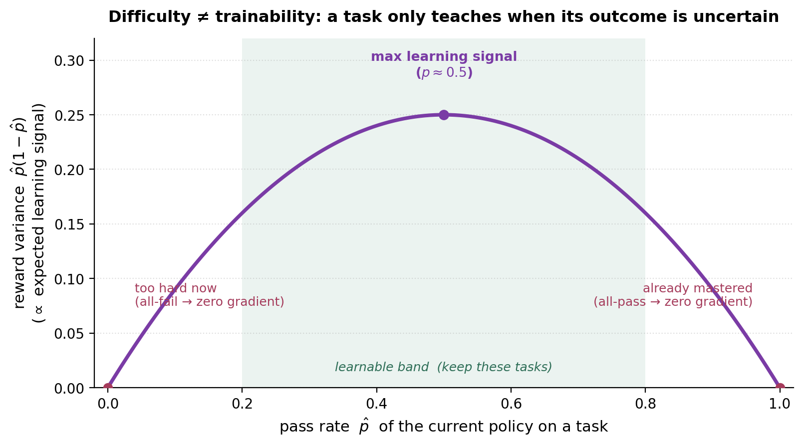 Reward variance \(\hat{p}(1-\hat{p})\) is maximized at \(p\approx0.5\) and zero at the extremes. A task the model always fails (\(p=0\)) or always passes (\(p=1\)) yields zero advantage and zero gradient — it teaches nothing right now, regardless of how “hard” it is in absolute terms.
Question: Why do people say agentic RL is “bottlenecked by environments, not algorithms”?
🎯 Because the algorithms (GRPO/PPO) are mature and cheap to apply, but RL is hungry for verifiable, interactive tasks, and hand-built benchmarks are tiny and evaluation-only. The scarce resource is executable, verifiable environments at scale — so most recent progress comes from generating them.
A benchmark like a few hundred coding or tool-use tasks is built to measure a model; RL burns through tasks far faster than humans can author them, and needs interactive tasks with a programmatic verifier (not just input/output pairs). So the lever that moves the needle is the supply of environments — procedurally generating containerized tasks and synthesizing their verifiers — rather than another tweak to the loss. This is the entire premise of the environment-scaling literature (companion post).
Question: Why isn’t the hardest task the most useful to train on?
🎯 Because a task you always fail gives zero reward variance, hence zero advantage and zero gradient — the same as a task you always pass. Learning signal peaks where success is uncertain (\(p\approx0.5\)), not where difficulty is maximal.
This is the most counter-intuitive lever in the pipeline. With a binary reward, the expected policy gradient magnitude scales with \(p(1-p)\): maximal at \(p=0.5\), zero at \(p\in\{0,1\}\). A brutally hard task (current pass rate 0) and a trivial task (pass rate 1) are equally useless right now — both yield no gradient. The practical consequences:
- Filter by learnability, not difficulty — keep tasks in a “learnable band” (e.g. \(0.2<p<0.8\)), which is exactly DAPO’s dynamic sampling (drop all-pass/all-fail prompts, §8).
- Curriculum — as the policy improves, today’s learnable tasks become trivial; difficulty must rise with capability to keep \(p\) near the middle (self-evolving environments, companion post).
Insight box — “Filter by learning signal, not raw difficulty.” The most useful task is the one the model gets right about half the time — not the hardest one.
Case study — MGPO. VibeThinker’s MaxEnt-Guided Policy Optimization (MGPO) is a concrete version of this principle. For each prompt, it samples a group of rollouts, estimates empirical correctness \(p(q)\), and upweights prompts closest to maximum uncertainty (\(p(q)\approx0.5\)) while downweighting all-pass or all-fail prompts. In other words, it turns the learnability band into a prompt-level weighting scheme inside a GRPO-style objective (Xu et al., 2025). This is also why VibeThinker is a useful small-model case study: it makes diversity first, signal second operational rather than just philosophical.
A task can be learnable but still unsafe or invalid. A learnable task is not automatically a good training environment; the verifier and reset mechanics have to be trustworthy too.
| Dimension | Bad environment | Good environment |
|---|---|---|
| Verifiability | public tests only; shallow regex | hidden/adversarial tests; state-based verifier |
| Reset | state leaks across episodes | deterministic clean snapshot |
| Learnability | all-pass or all-fail | \(p\) in the learnable band |
| Diversity | template duplicates | compositional variation |
| Safety | unrestricted tool side effects | sandboxed, scoped tools |
| Cost | slow / flaky / non-deterministic | bounded timeout, reproducible execution |
Takeaway. Agentic RL’s binding constraint is the supply of verifiable interactive environments, and the key selection principle is trainability (reward variance \(p(1-p)\)) rather than raw difficulty — which is why dynamic sampling and curricula matter as much as the RL algorithm.
§15 — Agent safety: the verifier is not the only attack surface
Key concepts.
For normal RLHF, reward hacking mostly means exploiting a reward model or judge. For agentic RL, the attack surface is larger: the agent acts through tools, reads untrusted observations, changes external state, and may receive rewards from an environment that itself can be manipulated. The failure can be a reward hack, a verifier hack, a tool-use exploit, a prompt-injection exploit, a sandbox escape, or an irreversible side effect. This is why agent training and deployment need a security boundary, not just a better reward.
Agentic RL safety is best treated as constraints around the whole environment–tool–verifier loop: scoped credentials, sandboxed tools, read/write permission separation, deterministic resets, hidden tests, human approval for irreversible actions, and explicit logging of side effects. The verifier is only one component; the rest of the environment can still leak state or provide shortcuts. Tool outputs should be treated as observations, not instructions — this connects prompt injection to the loss-masking rule in §13.
| Risk | Example | Mitigation |
|---|---|---|
| Prompt injection | tool output says "ignore your policy" | isolate untrusted observations; instruction hierarchy |
| Data exfiltration | agent reads secrets from files / DB | scoped credentials; allowlists; redaction |
| Sandbox escape | generated code touches host/network | containers, seccomp, network controls |
| Irreversible side effects | deletes data, sends email, buys item | human gate; dry-run mode; reversible transactions |
| Verifier hacking | satisfies public tests without solving task | hidden/adversarial tests; multi-verifier checks |
| Environment leakage | state persists across episodes | deterministic reset; clean snapshots |
Question (added): How do you prevent agentic RL from learning unsafe tool-use behavior?
🎯 Constrain the action space and permissions before training, not after. Use sandboxed/scoped tools, hidden tests, deterministic resets, human gates for irreversible actions, and monitor side effects — the reward cannot be the only safety mechanism.
The safe design pattern is least privilege. The training environment should expose only the tools needed for the task, with scoped credentials and no ambient secrets; destructive tools run in dry-run or approval mode; tool outputs are marked as untrusted observations rather than instructions; and every episode resets to a clean snapshot. During training, log tool-call count, failed calls, timeout rate, side-effect rate, and any permission-denied events. If a model learns to get reward by exploiting the environment rather than doing the task, the fix is not just reward shaping — it is narrowing or hardening the environment.
Question (added): What is the difference between reward hacking, verifier hacking, and benchmark overfitting?
🎯 Reward hacking exploits the proxy objective; verifier hacking exploits the checker implementation; benchmark overfitting exploits repeated exposure to the evaluation distribution. In agentic RL they often overlap, but the mitigations differ.
- Reward hacking: the model maximizes a learned RM while true quality falls (§5).
- Verifier hacking: the model learns quirks of tests, regexes, judges, or environment state.
- Benchmark overfitting: the model is indirectly trained toward public/easy-to-leak eval tasks.
Mitigations: independent held-out environments, hidden/adversarial tests, contamination checks, periodic manual audits, and separating training generators from evaluation verifiers. This is the agentic version of “do not train on the test set” — except the test set is executable and easier to accidentally leak.
Takeaway. In agentic RL, the verifier is not the only attack surface. The policy can exploit tools, state, permissions, and reset logic; safety starts with environment design and least-privilege tooling, then uses rewards and evals as additional checks.
Part VI — RL Infrastructure & Systems
§16 — Memory, parallelism, and precision
Key concepts.
A GRPO/PPO training step holds several copies of the model in memory at once. In the general PPO case: the policy (trained), a reference policy (for the KL term), a reward model, and a critic — up to four. GRPO removes the critic and the RM (verifiable reward), leaving policy + reference, and dropping the KL term removes the reference too — a major memory saving and a reason RLVR runs often drop KL (§8). On top of model weights you pay for optimizer states (Adam keeps two moments, so ~2× the parameter memory in fp32) and activations.
When a single copy does not fit, you shard. The axes:
- Data parallel / FSDP / ZeRO — replicate the computation across GPUs over different data; FSDP/ZeRO shard parameters, gradients, and optimizer states across ranks and gather them on demand (Rajbhandari et al., 2019; Zhao et al., 2023).
- Tensor parallel (TP) — split individual matmuls across GPUs (intra-layer) (Shoeybi et al., 2019, Megatron-LM).
- Pipeline parallel (PP) — split layers into stages across GPUs (inter-layer); avoided at moderate scale because of pipeline bubbles and complexity.
- Context parallel (CP) — split the sequence across GPUs for long context.
- Expert parallel (EP) — for MoE, place different experts on different GPUs.
Question (Infra-1): Without CPU offload, how many models are in memory during GRPO, and how much can you save?
🎯 Up to three with KL: policy + reference + (if learned-reward) reward model; GRPO already drops the critic. Dropping the KL term removes the reference model; using a verifiable reward removes the reward model — so a lean RLVR-GRPO run keeps essentially just the policy (plus optimizer states and the inference copy).
Accounting for a GRPO run: the policy (trainable, + optimizer states + activations) is the big cost; a reference copy (frozen, inference-only) is needed only for the KL penalty; a reward model (frozen) only if the reward is learned. The savings levers: drop KL ⇒ no reference model; verifiable reward ⇒ no reward model; quantize/shard the frozen copies (the reference/RM are inference-only, so they can be low-precision and sharded). What you cannot avoid is a serving copy of the policy for rollouts (§17) — in colocated setups it shares weights with the trainer; in disaggregated setups it is a separate, often quantized, replica.
Question (Algo-9): In LLM training, if you accidentally All-Reduce the loss a few extra times, what happens?
🎯 Data-parallel All-Reduce averages gradients across ranks; reducing the loss/gradient extra times (or summing instead of averaging) rescales the effective gradient — e.g. multiplying it by the world size — which is equivalent to blowing up the learning rate and typically destabilizes or diverges training.
In data-parallel training each rank computes a local gradient and a single All-Reduce averages them. If the loss (or its gradient) is All-Reduced an extra time, or summed rather than mean-reduced, the gradient gets scaled by a constant (often the number of ranks). Gradient scaling is identical to scaling the learning rate, so the update becomes far too large — loss spikes, NaNs, or silent divergence. It is a classic distributed-training bug: the math looks fine locally but the effective step size is multiplied by the world size. The fix is to ensure the loss is reduced exactly once with the correct mean reduction (and that gradient-accumulation normalization matches).
Question (Infra-3): INT8 vs FP8 — which for training, which for inference, and why?
🎯 FP8 for training, INT8 for inference. FP8 spends bits on a floating-point exponent, giving the dynamic range gradients/activations need; INT8 is fixed-point with more precision in a narrow range, which suits inference weights/activations after calibration.
Training values (gradients, activations) span a wide dynamic range, so you need an exponent — FP8 (e.g. E4M3/E5M2) keeps range at low precision and is now standard for large-model training (Peng et al., 2023, FP8-LM). Inference, especially weight quantization, tolerates fixed-point INT8 because the range is known and can be calibrated, and INT8 gives more mantissa precision within that range plus broad hardware support. Rule of thumb: FP8 = range (training); INT8 = precision-in-range (inference serving).
Question (Infra-10/11): Why is expert parallelism central for MoE, and how do Megatron and FSDP differ for long context?
🎯 MoE puts different experts on different GPUs (EP); routing then needs all-to-all communication to send each token to its expert, so throughput hinges on overlapping that all-to-all with compute and on expert load balance. For long context, FSDP shards parameters/optimizer states (simple, comms on demand) while Megatron uses explicit 3-D (TP+PP+DP) parallelism, adding context/sequence parallelism to split the sequence.
A MoE layer only activates a few experts per token, so the experts are sharded across GPUs (EP). The cost is an all-to-all to route tokens to their experts and back; throughput depends on (1) overlapping all-to-all with compute and (2) load balance (a hot expert stalls everyone). For long context, the activation/KV memory grows with sequence length, so you add context/sequence parallelism; FSDP keeps things simple (shard params/grads/optimizer, all-gather on demand, overlap comms with compute), while Megatron composes explicit TP × PP × DP (+ CP) for maximum control at large scale. FSDP is easier to use; Megatron extracts more performance at the cost of complexity.
Takeaway. Know where the memory goes (policy + optimizer states + frozen reference/RM copies) and what each parallelism axis splits (data/params: FSDP/ZeRO; matmuls: TP; layers: PP; sequence: CP; experts: EP). The cheapest RLVR memory win is dropping KL/RM; the classic correctness bug is mis-reduced gradients.
§17 — Rollout engines and serving
Key concepts.
In RL the bottleneck is usually generation, not the gradient update: every step needs fresh rollouts from the current policy, and autoregressive decoding is slow. So RL training leans on production inference engines. Two ideas dominate:
- Continuous batching — instead of waiting for a whole batch to finish, the scheduler swaps finished sequences out and new ones in at the token level, keeping the GPU busy (Yu et al., 2022, Orca).
- KV-cache management — the attention KV cache dominates inference memory; how you store and reuse it sets throughput. vLLM introduced PagedAttention, paging the KV cache like virtual memory to cut fragmentation (Kwon et al., 2023); SGLang introduced RadixAttention, sharing KV across requests with a common prefix via a radix tree (Zheng et al., 2023, SGLang).
A further systems pattern is disaggregated prefill/decode: prefill (compute-bound) and decode (memory-bandwidth-bound) have different profiles, so splitting them onto different GPUs and transferring the KV cache between them improves utilization (Zhong et al., 2024, DistServe).
Question (Infra-5): What problems does continuous batching cause in RL training, and how do vLLM and SGLang differ?
🎯 Continuous batching makes sequences in a batch finish at different times, so you must align completed trajectories and their log-probs before the training step — and the generation log-probs may not match the trainer’s (see §18). vLLM optimizes KV memory with PagedAttention; SGLang optimizes shared prefixes with RadixAttention — both speed rollouts but differ in what they cache.
In RL you generate a group of trajectories, then do a gradient step — so variable finish times mean straggler trajectories hold up the batch (the long-tail problem below) and you must carefully gather each sequence’s tokens and log-probs. The engines help differently: vLLM/PagedAttention is about memory (no KV fragmentation ⇒ bigger batches), while SGLang/RadixAttention is about reuse (shared prompt prefixes computed once ⇒ great when many rollouts share a prompt, exactly the RL group-sampling case). Many RL stacks use either as the rollout engine behind the trainer.
Question (Infra-4): What is the long-tail problem in RL rollouts, and how do you handle it?
🎯 Within a batch, a few trajectories run much longer than the rest (long generations, many tool turns), and a synchronous trainer must wait for the slowest — wasting GPUs. Fixes: continuous batching, length caps / early truncation, and asynchronous rollout so the trainer never blocks on stragglers.
A synchronous RL step is only as fast as its slowest rollout, and generation length is heavy-tailed (some problems induce very long chains or many tool calls). Mitigations: continuous batching (refill freed slots), truncation / max-turn limits (cap the tail, at the cost of dropping some signal), PipelineRL-style overlap of generation and training, and — most fundamentally — asynchronous RL (§18) that decouples rollout workers from the trainer so stragglers don’t stall the optimizer.
Question (Infra-6): How do you read utilization in vLLM/SGLang, and KV-cache utilization during training?
🎯 Track throughput (tokens/s), GPU compute utilization, and KV-cache occupancy (fraction of cache blocks in use, and how often requests are preempted/evicted). Low GPU util with low KV occupancy ⇒ you’re waiting (sync/CPU/scheduling); high KV occupancy with evictions ⇒ memory-bound, reduce batch or context.
The engines expose scheduler/cache metrics: throughput (tok/s), KV-cache occupancy (used blocks / total; PagedAttention/RadixAttention report this), running vs waiting/preempted requests, and GPU utilization. Diagnosis: low GPU util usually means you’re bound on something other than compute — rollout↔trainer synchronization, CPU work, or scheduling — rather than the model being slow; high KV occupancy with frequent evictions/preemptions means you’re memory-bound and should shrink batch size or max sequence length. In RL specifically, watch whether the trainer is idle waiting for rollouts — that idleness is the headline inefficiency async frameworks (§18) target.
Takeaway. Generation is the RL bottleneck; continuous batching plus KV-cache engines (vLLM’s PagedAttention for memory, SGLang’s RadixAttention for prefix reuse) are the main levers, and the long-tail of slow rollouts is what pushes systems toward asynchrony.
§18 — Async RL and training–inference consistency
Key concepts.
Synchronous RL alternates “generate a batch → update once,” so the trainer sits idle during generation and waits on the slowest rollout (§17). Asynchronous RL decouples rollout workers (many inference replicas, always generating) from the trainer (always updating), connected by a queue. This keeps both busy and is the basis of modern systems (AReaL Fu et al., 2025; slime, THUDM; verl Sheng et al., 2024; prime-rl). The price is off-policyness: rollouts are produced by a policy a few steps behind the trainer.
Staleness quantifies that gap — how many trainer updates behind the rollout-generating policy is. Bounded staleness (typically a few steps) plus an importance-sampling correction keeps async training close to on-policy; let it grow and the IS ratios explode and training destabilizes (§2, §7). This is the same “trust region” budget as PPO/TRPO, enforced over wall-clock instead of per-update.
A second, subtler problem is training–inference mismatch (训推不一致): the rollout engine and the trainer compute different probabilities for the same tokens, so the log-probs the rollouts were generated with don’t match what the trainer thinks — which corrupts the importance ratios. Causes: different kernels/engines (vLLM vs the training framework), quantization, reduction order, and — for MoE — different expert routing between inference and training. The fix is to make the two numerically consistent: batch-invariant kernels, matched reduction order, recompute log-probs on the trainer side, and replay the inference router’s expert choices (Thinking Machines Lab, 2025).
Question (Infra-8): What async RL frameworks exist, and what problem do they solve over synchronous training?
🎯 AReaL, slime, verl, prime-rl and similar decouple rollout generation from the gradient update so the trainer never idles waiting for (slow or straggling) rollouts — solving the GPU-underutilization and long-tail problems of synchronous RL, at the cost of off-policy staleness that must be controlled.
Synchronous RL wastes the trainer’s GPUs during generation and is hostage to the slowest rollout. Async frameworks run a pool of inference replicas continuously, feed a stream of trajectories to the trainer, and let the trainer update continuously. The new burden is bounding staleness and correcting the residual off-policyness with importance sampling — which is exactly what these frameworks instrument.
Question (Infra-14): What is full-async staleness, and roughly how stale do runs go?
🎯 Staleness = the number of trainer updates between the policy that generated a rollout and the current policy. Fully-async runs typically keep it small — on the order of 1–4 steps — because larger gaps make importance-sampling ratios unreliable and destabilize training.
In a fully-async setup, by the time a trajectory finishes and reaches the trainer, the policy has already moved on by some number of updates — that lag is staleness. Practically it is kept to a few steps (and hard-bounded): the IS correction \(\pi_\theta/\pi_{\text{behavior}}\) is only well-behaved when the two policies are close, so frameworks either cap the maximum off-policy steps or drop/down-weight too-stale samples (Fu et al., 2025).
Question (Infra-12): How do you turn on determinism, what is batch-invariance, what causes nondeterminism, and can atomic-add fix it?
🎯 Nondeterminism comes mostly from floating-point non-associativity under parallel reductions whose order varies with batching/scheduling (including atomic-add accumulation order). “Batch-invariant” kernels force the same reduction order regardless of batch size/shape so a token’s logprob is identical in any batch. Atomic-adds are a *cause (nondeterministic accumulation order), not a fix; determinism needs fixed-order reductions, not more atomics.*
Floating-point addition isn’t associative, so summing the same numbers in a different order gives slightly different results. GPU kernels reduce in parallel and the order depends on batch size, sequence packing, and scheduling — so the same token can get a slightly different logit in different batches. Atomic-add accumulation is one source: its completion order is nondeterministic, so it causes run-to-run variance rather than fixing it. The remedy is batch-invariant / deterministic kernels that fix the reduction order (and matching settings between the inference and training paths), so logprobs are reproducible and the training–inference mismatch shrinks (Thinking Machines Lab, 2025).
Question (Algo-11): What algorithms address MoE training–inference mismatch, and how?
🎯 Two complementary fixes: (1) make the importance ratio robust to per-token routing noise by moving it to the sequence level (GSPO); (2) make inference and training numerically consistent — replay the inference engine’s expert-routing decisions on the trainer side and use batch-invariant kernels so the same tokens get the same expert and the same probability.
MoE routing means a token’s probability depends on which experts fired, and that choice can differ between the rollout engine and the trainer (different kernels/scheduling), so the behavior-policy log-probs the rollouts carry don’t match the trainer’s recomputation — importance ratios become wrong. Mitigations: GSPO (§8) computes the importance ratio at the sequence level, which is far less sensitive to per-token routing noise than token-level ratios; and on the systems side, replay the router’s expert selection from inference and use deterministic/batch-invariant kernels so routing and probabilities line up (Thinking Machines Lab, 2025).
Question (Infra-9): In partial-rollout frameworks, do rollout workers keep the old policy’s KV cache?
🎯 KV cache is request-local and policy-version-specific. You generally do not reuse stale KV for training logprobs. A partial rollout may continue generation under the same behavior policy/version, but the trainer must know the saved behavior logprobs and policy version.
The KV cache stores intermediate keys/values for a specific model state and prefix. If the policy changes, the cache is no longer a faithful cache for the new policy. In practice, rollout workers may continue a partially completed trajectory under the same behavior policy that started it, but the training step should use the saved old logprobs (or recompute them with the matching behavior checkpoint) and tag the trajectory with its policy version. Do not use a stale cache to pretend the trajectory was generated by the current train policy.
Question (Infra-7): How is backprop done in multi-node multi-GPU RL training?
🎯 Rollout is inference; training is ordinary distributed backprop on the policy loss. The RL-specific part is assembling trajectories, logprobs, masks, rewards, and advantages; gradients are then reduced or sharded by DP/FSDP/ZeRO/TP/PP just like other LLM training.
The trainer receives a batch of tokens plus masks, old logprobs, advantages, and rewards. It recomputes new logprobs under the train policy, forms the clipped policy-gradient loss, backpropagates through the policy-generated tokens only, and synchronizes gradients according to the chosen parallelism: FSDP/ZeRO for parameter/optimizer sharding, tensor parallel for matmuls, pipeline parallel for layers, context parallel for long sequences. RL changes the data assembly and loss, not the fundamental backprop algorithm.
Question (Infra-16): VeRL / TRL / Unsloth / AReaL / slime — which would you choose?
🎯 Depends on scale and goal: TRL/Unsloth for single-node SFT/DPO and quick experiments (Unsloth for memory-efficient fine-tuning); VeRL as the general-purpose, scalable RL framework (HybridFlow design, strong engine integrations); AReaL/slime when you specifically need large-scale fully-async RL with staleness control. Choose by (1) sync vs async need, (2) scale, (3) engine integration.
A practical decision guide:
- TRL — Hugging Face’s library; great for SFT/DPO/PPO at small–medium scale, easy to start.
- Unsloth — memory/throughput-optimized fine-tuning (LoRA/QLoRA); single-GPU/-node efficiency.
- VeRL — scalable RLHF/RLVR with a HybridFlow controller and vLLM/SGLang + FSDP/Megatron backends (Sheng et al., 2024); a common default for serious RL.
- AReaL — fully-asynchronous RL with explicit staleness control (Fu et al., 2025).
- slime (THUDM) — Megatron-backed RL framework focused on rollout throughput.
There is no universal best; match the framework to sync-vs-async, scale, and which inference/ training backends you need.
Takeaway. Async RL trades synchronous simplicity for utilization, introducing staleness (bounded + IS-corrected) and training–inference mismatch (fixed via numerical consistency: batch-invariant kernels, replayed routing, trainer-side logprobs). For MoE, GSPO plus routing replay are the key levers; framework choice follows from sync/async, scale, and backend needs.
§19 — Summary, cheat-sheet, and further reading
The one-paragraph version. Post-training turns a base model into a useful one through a recipe — SFT, reward modeling, rejection sampling, RL, and direct-alignment/distillation — whose central fork is learned reward (RLHF) vs verifiable reward (RLVR). The RL core is policy-gradient/actor-critic: LLMs need an explicit policy for stochastic, sequence-level generation with sparse trajectory rewards; PPO approximates a trust region by clipping; GRPO drops the critic for a group baseline; DPO skips the loop entirely with an implicit reward. Rewards are the attack surface — verifiable ones shrink it, KL bounds drift, nothing is unhackable. Evaluation is what tells you whether reward gains became real capability rather than proxy overfit. RLVR elicits reasoning that mostly already exists in the base model (pass@1 ↑, pass@k ≈), and exploration/entropy is the limiting resource. Agentic RL stretches all of this over tool-interleaved trajectories, where the binding constraints become credit assignment, environment supply, trainability (reward variance \(p(1-p)\)), and safety boundaries around tools and side effects. And at scale RL is a systems problem: memory (how many model copies), generation throughput (rollout engines), and the off-policyness + training–inference mismatch that async training introduces.
Algorithm cheat-sheet.
| Method | One-line | Critic? | Reward | Use when |
|---|---|---|---|---|
| REINFORCE | raw policy gradient | no | any | pedagogy; rarely alone |
| PPO | clipped trust region, actor+critic | yes | RM or verifiable | general RLHF |
| GRPO | group-mean baseline, no critic | no | usually verifiable | RLVR/reasoning at scale |
| Dr. GRPO | GRPO minus std/length bias | no | verifiable | cleaner GRPO |
| DAPO | clip-higher + dynamic sampling + token loss, drop KL | no | verifiable | aggressive reasoning RL |
| GSPO | sequence-level IS ratio | no | verifiable | MoE stability |
| CISPO | clip the IS weight, keep all-token gradient | no | verifiable | long-CoT / MoE |
| DPO | offline preference loss, implicit reward | no | preference pairs | cheap alignment, no RM/rollouts |
Hyperparameter defaults (GRPO). group size 8–16 · lr ~1e-6 · PPO epochs ≈1 · generation length to task. Systems quick-ref. Parallelism: FSDP/ZeRO (data/params) · TP (matmuls) · PP (layers) · CP (sequence) · EP (experts). Rollout engines: vLLM (PagedAttention, memory) · SGLang (RadixAttention, prefix reuse). Frameworks: TRL/Unsloth (small) · VeRL (general scalable) · AReaL/slime (async at scale).
The mental model. Reward defines the goal; the algorithm bounds how fast you chase it; the environment supplies the experience; the systems make it fast; and consistency (clip, KL, staleness, numerics) keeps it from blowing up.
Further reading
- Nathan Lambert, RLHF Book — the canonical recipe-organized reference (rlhfbook.com).
- wh, SFT, RL, and On-Policy Distillation Through a Distributional Lens — a useful intuition for when to stop SFT and why on-policy data matters (blog).
- WeiboAI, VibeThinker-1.5B / 3B — compact reasoning models that operationalize spectrum-first SFT and trainability-weighted RL (GitHub, 1.5B HF, 3B HF).
- The companion post, Environment Scaling for Agentic RL — how environments are synthesized at scale.
- Primary papers per section are linked inline and collected in References.
- Source question set: “RL Interview Questions 2026” (@sheriyuo; zhihu).
Living document. This post is maintained over time: new questions, citations, and open problems can be added as they show up in interviews and papers. Corrections welcome.
Open questions (tracked, to expand)
- Can exploration-preserving, prolonged RL expand the capability frontier, or only sharpen it? (§10–§11)
- Process rewards vs outcome rewards for long-horizon agents — when is densifying credit worth the added attack surface? (§13)
- Principled curricula for trainability (keeping \(p\approx0.5\)) as the policy improves. (§14)
- Eliminating training–inference mismatch for MoE without sacrificing throughput. (§18)
- The right abstraction for verifiable rewards beyond math/code (open-ended, multi-step, tool-using tasks). (§5, §14)
Appendix — The source interview questions
This post is organized by concept, but it grew out of a concrete interview question set — “RL Interview Questions 2026” by @sheriyuo (zhihu version). For readers using this as interview prep, here is the original list with a pointer to where each is answered. Treat it as a self-test checklist: can you answer each in 60 seconds?
Algorithm
- Why use actor-critic rather than a pure critic? → §3
- How do KL divergence, cross-entropy, and MLE relate? → §2
- How should you design rewards for different RL settings? → §5
- Importance sampling / rejection sampling / Monte-Carlo in RL? → §2
- How is the PPO/GRPO advantage computed; why subtract a baseline; must you divide by std? → §8
- How do RL training and test-time scaling each explore? → §11
- How does PPO clip; why the
min; what if you don’t clip; what is CISPO? → §7 - Why does GRPO add KL; how is it computed; why do DAPO/GSPO drop it? → §8 (computation also §5/§7)
- What happens if you accidentally All-Reduce the loss a few extra times? → §16
- What is DPO’s implicit reward; can the objective be over-optimized or exploited; how do you fix it? → §9
- Algorithms for MoE training–inference mismatch, and their principles? → §18
- How to set group size / learning rate / PPO epochs / generation length? → §8
- How do Dr.GRPO / DAPO / GSPO / CISPO improve on GRPO, and their weaknesses? → §8
- How do TRPO / PPO / AReaL constrain the RL objective with a trust region? → §7 (+§18)
- Can RL expand an LLM’s capability boundary? → §10
- How do you scale the RL training frontier (cf. ProRL)? → §11
- How does on-policy distillation improve on RL / SFT; its applications? → §6
- At which training stage does reasoning ability emerge? → §10
- From DeepSeek-R1 to V3.2/V4: RL changes, and how MoE-RL differs? → §11 (+§18)
Infrastructure
- Without CPU offload, how many models are in memory during GRPO; how much can you save? → §16
- Distributed inference: KV-cache transfer and multi-GPU communication optimization? → §17
- INT8 vs FP8 trade-offs; which precision for training vs inference? → §16
- What is the long-tail problem in RL rollouts; solutions? → §17
- Problems with continuous batching in RL; vLLM vs SGLang? → §17
- Reading utilization in vLLM/SGLang and KV-cache utilization in training? → §17
- How is backprop done in multi-node multi-GPU RL training? → §16 (+§18)
- What async RL frameworks exist; what synchronous-training problem do they solve? → §18
- Do partial-rollout frameworks (AReaL etc.) keep the previous policy’s KV cache? → §18
- How does MoE expert parallelism affect throughput? → §16
- Long-context compute–communication overlap; Megatron vs FSDP parallelism? → §16
- Determinism mode, batch-invariance, what causes it, and atomic-add? → §18
- How do AReaL and slime differ in understanding the rollout bottleneck? → §18
- What is full-async staleness, and roughly how large in practice? → §18
- In slime / Megatron-backed RL frameworks, what should you understand at a high level? → §18 (framework choice)
- VeRL / TRL / Unsloth / AReaL / slime — which would you choose? → §18
References
(Inline citations throughout link directly to sources; this is the consolidated list.)
[1] Ronald J. Williams. “Simple Statistical Gradient-Following Algorithms for Connectionist Reinforcement Learning.” Machine Learning, 1992.
[2] Richard S. Sutton, David McAllester, Satinder Singh, Yishay Mansour. “Policy Gradient Methods for Reinforcement Learning with Function Approximation.” NeurIPS, 2000.
[3] John Schulman, Sergey Levine, Philipp Moritz, Michael I. Jordan, Pieter Abbeel. “Trust Region Policy Optimization.” ICML, 2015. arXiv:1502.05477.
[4] John Schulman, Philipp Moritz, Sergey Levine, Michael I. Jordan, Pieter Abbeel. “High-Dimensional Continuous Control Using Generalized Advantage Estimation.” ICLR, 2016. arXiv:1506.02438.
[5] John Schulman, Filip Wolski, Prafulla Dhariwal, Alec Radford, Oleg Klimov. “Proximal Policy Optimization Algorithms.” arXiv:1707.06347, 2017.
[6] Nisan Stiennon, Long Ouyang, Jeff Wu, et al. “Learning to Summarize from Human Feedback.” NeurIPS, 2020. arXiv:2009.01325.
[7] Long Ouyang, Jeff Wu, Xu Jiang, et al. “Training Language Models to Follow Instructions with Human Feedback” (InstructGPT). NeurIPS, 2022. arXiv:2203.02155.
[8] Nathan Lambert. “Reinforcement Learning from Human Feedback” (RLHF Book). Online, 2026.
[9] Wei Fu, Jiaxuan Gao, Xujie Shen, et al. “AReaL: A Large-Scale Asynchronous Reinforcement Learning System for Language Reasoning.” arXiv:2505.24298, 2025.
[10] MiniMax. “MiniMax-M1: Scaling Test-Time Compute Efficiently with Lightning Attention” (introduces CISPO). arXiv:2506.13585, 2025.
[11] Zhihong Shao, Peiyi Wang, Qihao Zhu, et al. “DeepSeekMath: Pushing the Limits of Mathematical Reasoning in Open Language Models” (introduces GRPO). arXiv:2402.03300, 2024.
[12] DeepSeek-AI. “DeepSeek-R1: Incentivizing Reasoning Capability in LLMs via Reinforcement Learning.” arXiv:2501.12948, 2025.
[13] John Schulman. “Approximating KL Divergence” (the k1/k2/k3 estimators). Blog, 2020.
[14] Zichen Liu, Changyu Chen, Wenjun Li, et al. “Understanding R1-Zero-Like Training: A Critical Perspective” (Dr. GRPO). arXiv:2503.20783, 2025.
[15] Qiying Yu, Zheng Zhang, Ruofei Zhu, et al. “DAPO: An Open-Source LLM Reinforcement Learning System at Scale.” arXiv:2503.14476, 2025.
[16] Qwen Team. “Group Sequence Policy Optimization.” arXiv:2507.18071, 2025.
[17] Rafael Rafailov, Archit Sharma, Eric Mitchell, et al. “Direct Preference Optimization: Your Language Model is Secretly a Reward Model.” NeurIPS, 2023. arXiv:2305.18290.
[18] Mohammad Gheshlaghi Azar, Mark Rowland, Bilal Piot, et al. “A General Theoretical Paradigm to Understand Learning from Human Preferences” (IPO). arXiv:2310.12036, 2023.
[19] Kawin Ethayarajh, Winnie Xu, Niklas Muennighoff, et al. “KTO: Model Alignment as Prospect Theoretic Optimization.” arXiv:2402.01306, 2024.
[20] Yu Meng, Mengzhou Xia, Danqi Chen. “SimPO: Simple Preference Optimization with a Reference-Free Reward.” NeurIPS, 2024. arXiv:2405.14734.
[21] Richard S. Sutton, Andrew G. Barto. “Reinforcement Learning: An Introduction” (2nd ed.). MIT Press, 2018.
[22] Jason Wei, Maarten Bosma, Vincent Y. Zhao, et al. “Finetuned Language Models Are Zero-Shot Learners” (FLAN). ICLR, 2022. arXiv:2109.01652.
[23] Nathan Lambert, Jacob Morrison, Valentina Pyatkin, et al. “Tülu 3: Pushing Frontiers in Open Language Model Post-Training” (popularizes “RLVR”). arXiv:2411.15124, 2024.
[24] Hugo Touvron, Louis Martin, Kevin Stone, et al. “Llama 2: Open Foundation and Fine-Tuned Chat Models” (rejection-sampling fine-tuning). arXiv:2307.09288, 2023.
[25] Ralph A. Bradley, Milton E. Terry. “Rank Analysis of Incomplete Block Designs: I. The Method of Paired Comparisons.” Biometrika, 1952.
[26] Lianmin Zheng, Wei-Lin Chiang, Ying Sheng, et al. “Judging LLM-as-a-Judge with MT-Bench and Chatbot Arena.” NeurIPS, 2023. arXiv:2306.05685.
[27] Yuntao Bai, Saurav Kadavath, Sandipan Kundu, et al. “Constitutional AI: Harmlessness from AI Feedback.” arXiv:2212.08073, 2022.
[28] Dario Amodei, Chris Olah, Jacob Steinhardt, et al. “Concrete Problems in AI Safety.” arXiv:1606.06565, 2016.
[29] Joar Skalse, Nikolaus H. R. Howe, Dmitrii Krasheninnikov, David Krueger. “Defining and Characterizing Reward Hacking.” NeurIPS, 2022. arXiv:2209.13085.
[30] Leo Gao, John Schulman, Jacob Hilton. “Scaling Laws for Reward Model Overoptimization.” ICML, 2023. arXiv:2210.10760.
[31] Rishabh Agarwal, Nino Vieillard, Yongchao Zhou, et al. “On-Policy Distillation of Language Models: Learning from Self-Generated Mistakes” (GKD). ICLR, 2024. arXiv:2306.13649.
[32] Jason Wei, Xuezhi Wang, Dale Schuurmans, et al. “Chain-of-Thought Prompting Elicits Reasoning in Large Language Models.” NeurIPS, 2022. arXiv:2201.11903.
[33] Yang Yue, Zhiqi Chen, Rui Lu, et al. “Does Reinforcement Learning Really Incentivize Reasoning Capacity in LLMs Beyond the Base Model?” arXiv:2504.13837, 2025.
[34] Mingjie Liu, Shizhe Diao, et al. “ProRL: Prolonged Reinforcement Learning Expands Reasoning Boundaries in Large Language Models.” arXiv:2505.24864, 2025.
[35] Daixuan Cheng, Shaohan Huang, Xuekai Zhu, et al. “Reasoning with Exploration: An Entropy Perspective.” arXiv:2506.14758, 2025 / AAAI 2026.
[36] Ganqu Cui, Yuchen Zhang, Jiacheng Chen, et al. “The Entropy Mechanism of Reinforcement Learning for Reasoning Language Models.” arXiv:2505.22617, 2025.
[37] Niklas Muennighoff, Zitong Yang, Weijia Shi, et al. “s1: Simple Test-Time Scaling.” arXiv:2501.19393, 2025.
[38] DeepSeek-AI. “DeepSeek-V3.2: Pushing the Frontier of Open Large Language Models.” arXiv:2512.02556, 2025.
[39] DeepSeek-AI. “DeepSeek-V4: Towards Highly Efficient Million-Token Context Intelligence.” arXiv:2606.19348, 2026.
[40] DeepSeek. “Transparency Center.” 2026.
[41] NVIDIA NIM. “deepseek-v4-pro Model Card.” 2026.
[42] Samyam Rajbhandari, Jeff Rasley, Olatunji Ruwase, Yuxiong He. “ZeRO: Memory Optimizations Toward Training Trillion Parameter Models.” SC, 2020. arXiv:1910.02054.
[43] Yanli Zhao, Andrew Gu, Rohan Varma, et al. “PyTorch FSDP: Experiences on Scaling Fully Sharded Data Parallel.” VLDB, 2023. arXiv:2304.11277.
[44] Mohammad Shoeybi, Mostofa Patwary, Raul Puri, et al. “Megatron-LM: Training Multi-Billion Parameter Language Models Using Model Parallelism.” arXiv:1909.08053, 2019.
[45] Houwen Peng, Kan Wu, Yixuan Wei, et al. “FP8-LM: Training FP8 Large Language Models.” arXiv:2310.18313, 2023.
[46] Gyeong-In Yu, Joo Seong Jeong, Geon-Woo Kim, et al. “Orca: A Distributed Serving System for Transformer-Based Generative Models” (continuous batching). OSDI, 2022.
[47] Woosuk Kwon, Zhuohan Li, Siyuan Zhuang, et al. “Efficient Memory Management for Large Language Model Serving with PagedAttention” (vLLM). SOSP, 2023. arXiv:2309.06180.
[48] Lianmin Zheng, Liangsheng Yin, Zhiqiang Xie, et al. “SGLang: Efficient Execution of Structured Language Model Programs” (RadixAttention). NeurIPS, 2024. arXiv:2312.07104.
[49] Yinmin Zhong, Shengyu Liu, Junda Chen, et al. “DistServe: Disaggregating Prefill and Decoding for Goodput-optimized LLM Serving.” OSDI, 2024. arXiv:2401.09670.
[50] Guangming Sheng, Chi Zhang, Zilingfeng Ye, et al. “HybridFlow: A Flexible and Efficient RLHF Framework” (verl). EuroSys, 2025. arXiv:2409.19256.
[51] Horace He, Thinking Machines Lab. “Defeating Nondeterminism in LLM Inference.” Blog, 2025.
[52] Sen Xu, Yi Zhou, Wei Wang, et al. “Tiny Model, Big Logic: Diversity-Driven Optimization Elicits Large-Model Reasoning Ability in VibeThinker-1.5B.” arXiv:2511.06221, 2025.
[53] Sen Xu, Shixi Liu, Wei Wang, et al. “VibeThinker-3B: Exploring the Frontier of Verifiable Reasoning in Small Language Models.” arXiv:2606.16140, 2026.